


2019 Volume 2 Issue 2
|
|
INEOS OPEN, 2019, 2 (2), 55–67 Journal of Nesmeyanov Institute of Organoelement Compounds DOI: 10.32931/io1910a |
|


Microphase Separation of Amphiphilic Diblock Copolymers
under Cylindrical Confinement: a Strong Finite Size Effect
a Nesmeyanov Institute of Organoelement Compounds, Russian Academy of Sciences, ul. Vavilova 28, Moscow, 119991 Russia
b Chemistry Department, Lomonosov Moscow State University, Leninskie Gory, Moscow, 119991 Russia
Corresponding author: I. Ya. Erukhimovich, e-mail: ierukhs@polly.phys.msu.ru
Received 11 December 2018; accepted 29 January 2019
Abstract
The ordering of amphiphilic diblock copolymers in the bulk and under cylindrical confinement is studied via Monte Carlo simulation both visually and based on the structure factor analysis. Depending on the temperature and block architecture, single spherical or cylindrical micelles, lamellae with parallel and mutually orthogonal layers, and bi-continuous structures appear in the bulk, whereas snapshots in cylinders reveal lamellar-catenoid and spiral motifs. The structure factor analysis strongly supports the preferred formation of bi-continuous phases of amphiphilic copolymers in the bulk. The notion of the sectoral structure factor is introduced to extract symmetry information on the structure of cylindrically confined polymers and to prove the ordering reduction in narrow capillaries.
Key words: amphiphilic copolymers, self-organization, structure factor.
Introduction
The purpose of the present work is to study some peculiarities of an order–disorder transition (ODT) in amphiphilic block copolymers confined in cylindrical capillaries.
One of the most appealing features of block copolymer macromolecules is that, upon an increase of incompatibility of their blocks, they can form (both in melts and in semidilute and concentrated solutions) spatially periodic morphologies, which possess various crystal symmetries. A transition from a spatially homogeneous to a spatially periodic morphology is called ODT or microphase separation. Even the simplest (relative to their architectures) melts of diblock copolymer macromolecules AnBm form (depending on their composition and temperature) body-centered cubic lattices of almost spherical micelles, planar hexagonal lattices of almost cylindrical micelles as well as lamellar and bi-continuous morphologies [1–7]. Some conditions for realization of an orthorhombic morphology with the space group Fddd symmetry were also found both theoretically [8, 9] and experimentally [10, 11] (for ternary ABC linear triblock copolymers). Alternating gyroid, diamond, simple cubic and monoclinic morphologies were found and studied for more complex architectures (ternary ABC, two-scale multi-block copolymers, etc.) both experimentally [11] and theoretically [12, 13].
The situation becomes even more complicated when ODT occurs under some spatial constraints [14–18]. In cylindrical pores, the type of emerging morphologies depends on the reduced capillary diameter κ = D/L (here L is the characteristic bulk period of the morphology and D is the pore diameter), which indicates how much a natural set of copolymer conformations is distorted under confinement. In the limit κ → ∞, bulk morphologies arise, but a decrease of κ can lead to new shapes that would replace the bulk morphologies, depending on the way the blocks interact with the pore walls as well as on the type of the morphology which would occur for the system under consideration in the bulk.
Upon a decrease of the reduced capillary diameter κ, the lamellar morphology of symmetric diblock copolymers can transform into coaxial AB alternating cylindrical shells, if the affinities of A and B blocks to the wall differ enough. Otherwise, a perpendicular lamella morphology, where the alternating layers are oriented perpendicular to the pore axes (some authors call this morphology also "stacked discs"), stays for any κ [19–24]. Asymmetric diblock copolymers in pores of finite diameter κ~1 can form stacked toroids, one-, double- and triple-stranded helices (with and without a central rod), catenoid-cylinder, stacked spheres, etc., depending on the relationship between the values of copolymer asymmetry, reduced surface field, temperature, and reduced capillary diameter κ [23–29].
In the present work, we consider the self-organization of diblock copolymers with linear Ak and grafted amphiphilic (А-graft-Bm)n parts in bulk and under cylindrical confinement (m = 2–4). These diblock copolymers with short (m = 1, 2) side chains have been already studied via computer simulation [30–32] and self-consistent field theory (SCFT) [33]. The morphologies arising upon strong incompatibility of units A and B were found to depend on the relationship between the lengths of two blocks. The stable lamellae arise for the much lower content of the amphiphilic block, than it would occur for the conventional diblock copolymers AnBm. In literature, (А-graft-B1)N model is often used to describe the so-called amphiphilic homopolymers [34], i.e., the macromolecules being amphiphilic at the level of single monomer units [35, 36]. The amphiphilic homopolymers demonstrate a distinct propensity to self-assembly and have attracted particular interest over recent years [37, 38].
Further presentation is organized as follows. In Section 2 we describe the model of an amphiphilic diblock copolymer and the Monte Carlo simulation routine applied. In Section 3 we summarize the known results on the bulk morphologies formed by amphiphilic diblock copolymers with different compositions. In the rest of the paper we present and discuss our results on morphologies of the amphiphilic diblock copolymer formed under cylindrical confinement. Section 4 starts with the description of cylindrically confined morphologies for the amphiphilic diblock copolymers with various compositions for two different capillary geometries via visual description of the corresponding snapshots. Since the morphologies seem to be much more complicated than the bulk ones, one needs a special technique to identify the cylindrical morphologies. Such a technique, which is nothing but the correlation function technique (CFT) extended recently to confined systems [39–41], is presented in Section 5 to define the order parameter, corresponding to the structural modes distinguishable under formation of cylindrical morphologies, and to characterize the self-assembly evolution in a computer modeling experiment. At last, in Section 6 we consider the radius depending "long-scale short ordering" that arises in narrow cylinders. The summary of the results is given in Conclusions.
2. Model and simulation technique
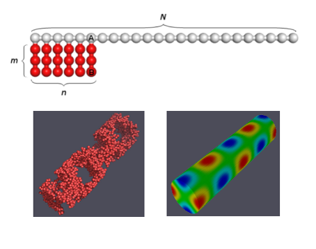
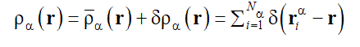
The model of amphiphilic macromolecules under consideration is presented schematically in Fig. 1.
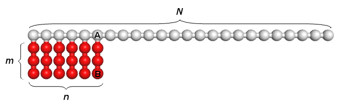
Figure 1. Schematic model of the studied macromolecules. N, n and m are the degrees of polymerization of the main chain, the amphiphilic block and the side chain. K = N + nm is the total degree of polymerization. The choice n = N, m = 1 corresponds to the original model [35] of the amphiphilic chain.
Each amphiphilic macromolecule is assumed to consist of a linear block Ak and a comb-like block (А-graft-Bm)n. In other words, a backbone of the macromolecule consists of N = k + n repeated units A, n of which contain engrafted side blocks Bm. To simulate the behavior of this system, we use the Monte Carlo method for the bond-fluctuation model (BFM) on the cubic lattice, which is known to provide a fairly fast convergence when modeling dense systems of branched macromolecules [42, 43]. Furthermore, for the capillary radii large enough compared to the distance a between the lattice nodes, that is the case in our calculations, the edge (finite size) corrections are negligible.
According to BFM, each unit occupies one elementary volume comprised of 8 lattice sites and we assume that the bond length can adopt values in the following range
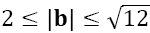
(hereinafter, we use the distance a between the nearest lattice nodes of the cubic lattice as the length unit).
Interaction between the units is described by a step-wise potential:
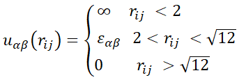 |
α, β = A, B, (1) |
where rij is the distance between two units, i-th and j-th, εαβ are the energy parameters, and α, β are the types (A, B) of repeated units. All the energies are expressed in terms of kT (k is the Boltzmann constant). The units of the same type interact only via the effect of excluded volume (εAA = εBB = 0), whereas unlike units A and B repel each other (εAB ≥ 0). More precisely, we set in our calculations 0 ≤ εAB ≤ 8.
In the standard Monte Carlo method, to make an elementary motion ("try") one selects randomly a unit and a neighboring site where the unit is supposed to be moved. The try is supposed to be allowable only if both the bond length restrictions and the self-avoidance condition are obeyed. Besides, a transition into a new conformation occurs according to the Metropolis criterion with the probability P = min{1, exp(−ΔE/kT)}, where ΔE = E2 – E1 and E1, E2 are the energies in the initial and new configurations, respectively.
To simulate ODT of the system in the bulk, we placed macromolecules into a cubic cell d×d×d with d = 64a and imposed the periodic boundary conditions along all three axes. Simulations were carried out for the chains comprising N = 24 units A in the backbone. The degree of polymerization of the amphiphilic block varied between n = 1 and n = N = 24. Each side chain of the amphiphilic block consisted of m ( 2 ≤ m ≤ 4) units B.
To provide equal volume fraction (ϕ ≈ 0.47) of macromolecules with different architectures within the computation cell with fixed size d×d×d, the total number M of chains in the cell is to be varied. Say, at m = 2, n = 1 (and, therefore, K = 26) the desired value of ϕ is achieved at M = 576 macromolecules, while at m = 2 and n = N = 24 (K = 72) one needs M = 216 chains. The volume fraction was chosen to reach the highest possible concentration of the polymer still keeping the convergence of the method, i.e., the sufficient mobility of the monomer units. An effective way to provide the high polymer concentration in a cell is to arrange the macromolecules regularly in the initial conformation and let them relax until they become distributed homogeneously [31]. More precisely, the initial configuration consisted of totally stretched chains distributed layer-wise into two columns. For the afore-mentioned example at m = 2, n = 1 and M = 576 there were 9 layers with 32 macromolecules per each layer and at m = 2, n = 24, M = 216 there were 6 layers each including 18 macromolecules. After the initial conformation had been built, the simulation was performed at εAB = 0 during 106 Monte Carlo steps to prepare a uniform mixture of macromolecules.
Next, we change the interaction parameter εAB gradually from 0 to 8 with the step equal to 0.5, the system being equilibrated during 1×10⁶ Monte Carlo steps at each value of εAB. The total energy is found to achieve its equilibrium value during this procedure.
To simulate in a capillary, macromolecules were placed into a cylindrical cell (pore) of the radius R and the length H. The periodic boundary conditions were imposed along the cylinder axis z.
Interaction of the units with the capillary wall was described via potential Uc:
 |
(2) |
where r is the distance between the monomer unit and the axis of capillary, εi is the energy of the units of the i-th type (i = A, B) in the boundary layer which we introduced due to some computational reasons, and d0 = 5 is the layer thickness.
In our calculations, we set εA = 0 and εB = 0 or εB = 4 (the wall is impenetrable for units of both A and B types and can selectively repel units B). The calculations were carried out for two different capillary lengths H = 64 and H = 128 and the radius R changing from 20 to 32. The number of macromolecules M in each experiment was chosen to provide the volume fraction of macromolecules as close to 0.5 as possible. The calculations were started from two different initial configurations with macromolecules placed in ordered layers perpendicular to the cylinder axis or parallel to it. The final results were found to be independent from the initial configuration.
3. Bulk morphologies of the amphiphilic diblock copolymers
Now we present the results of our simulations in the bulk for m = 3, 4 and compare them with the previous results [31, 33] for m = 1 and m = 2.
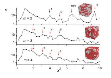
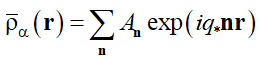
Let us first analyze the state of the systems studied visually (via characteristic snapshots). To begin with, we would like to remind a reader an earlier relationship [31] between the morphology and fraction of the amphiphilic units and AB repulsion for m = 2. The ordered morphologies arise when the unit incompatibility is still weak enough (εAB ~ 1) [31]. As incompatibility εAB increases, the ordering becomes more pronounced and boundaries between different domains become sharper. However, starting from εAB ≥ 2.0, the morphology practically does not change with a further increase of incompatibility up to εAB = 8. This feature is observed for m = 3, 4 as well. So, in further treatment we restrict the comparative analysis only to the composition dependence of the morphologies for εAB = 8. The corresponding snapshots are shown in Fig. 2.
a b
c d
e
Figure 2. Effective structure factors and typical snapshots for (a) n = 1, (b) n = 3, (c) n = 6, (d) n = 12, (e) n = 24, and εAB = 8. (a) m = 2, g0 = q*2 / q02 = 6; m = 3, g0 = 4; m = 4, g0 = 4. (b) m = 2, g0 = 4; m = 3, g0 = 4; m = 4, g0 = 3. (c) m = 2, g0 = 4; m = 3, g0 = 4; m = 4, g0 = 4. (d) m = 2, g0 = 4; m = 3, g0 = 5; m = 4, g0 = 5. (e) m = 2, g0 = 25; m = 3, g0 = 16; m = 4, g0 = 16. The dominant Bragg peaks (but the first one) are indicated by arrows. The numbers (if shown) specify the values of the relative squares of the coordination spheres corresponding to the peaks; unlabelled peaks are not considered to be reliable. The simulation data are given by the locations of symbols (■); the lines are guides for eyes.
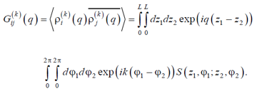
For the quantitative analysis, we consider the structure factors defined as follows:
Sαα (q) = < | ∫ drρα (r) exp(iqr) |2 > (3)
Here q is the scattering vector, the brackets <f> imply thermodynamic averaging of the quantity f over all states of the system studied, which is equivalent to time averaging (no ergodicity breaking is expected in our case) and an instant profile ρα(r) of the number density of the units of the α-th sort reads
 |
(4) |
In Eq. (4) is δρα (r) the fluctuating part (<| δρα (r) |> = 0) and  is the inhomogeneity that is thermodynamically stable as a result of microphase separation (ordering) and possesses the space group symmetry M :
 , (5)
, (5)
where q* = 2π/L is the characteristic scale of the reciprocal lattice corresponding to the group M and An is the complex amplitude. Summation in Eq. (5) is to be done over all vectors n, which are the radius-vectors of the nodes of the reciprocal lattice M with the unit radius of the first coordination sphere. Substituting the second of equalities (4), where rjα is the radius-vector of the j-th unit of the α-th type (α =A, B) and summation is taken over all Nα units of the chosen type α, into Eqs. (5) and (3), one gets
 |
(6) |
On the other hand, substituting the first of equalities (4) into Eq. (3), one gets
| (7) |
where Ãn = AnV, Δ(x) = 1 if x = 0 and Δ(x) = 0 otherwise. The first term in Eq. (7) describes the discrete Bragg diffraction peaks, whereas the second one does diffuse scattering on thermodynamic fluctuations. It should be reminded that the simulated scattering curves, which we calculated via expression (6) and presented in Fig. 2, correspond to the total (both for the structural and fluctuation) scattering.
For each structure, the static structure factors should be calculated. Thereby, one should have in mind that the structure factors in the bulk systems possessing crystal symmetry depend on both the modulus and direction of their continuous vector argument q. To simplify the presentation of the results, we calculate the angle average of the structure factors which we call further the effective structure factor:
|
|
(8) |
where α = B if the number of units A in the chain is higher than that of units B and α = A otherwise, x2 = (q/q*)2 is the reduced squared wave number, q* is the location of the first maximum on the effective structure factor dependence on the wave number q, and summation is to be done over all ν(x2) nodes of the reciprocal lattice under consideration, which belong to the coordination sphere with the radius  . Moreover, we calculated the effective structure factor every 102 steps in the course of 106 consecutive Monte Carlo steps and next averaged it over time and four independent runs. Thus, the information we extract from the structure factor is more representative than that from some the selected snapshots.
One more important remark concerns the fact that the wave vector q for a finite simulation box with the periodic boundary conditions is discrete:
q = q0 i, i = ( i1, i2, i3 ) (9)
where q0 = 2π/d and i1, i2, i3 are integers. Thus, the values of the argument x2 in Eq. (8) read  with g = i2 = 1,2,3,4,5,6,8,9,10,11,12,14...(for the cubic lattice) and
  . In the limit d → ∞, q0 → ∞, g0 → ∞, there would be no difference with the bulk behavior, but for our finite simulation box we find g0 = 3, g0 = 4, g0 = 5, g0 = 6, etc., depending on the values of n and m. So, the ratios of the discrete peaks' locations of σ(x2) in the finite simulation cell can differ noticeably from those in the bulk that indicate the occurrence of that or another crystal lattice, which leads to some additional problems in identification of the kind of crystal symmetry occurred. We return to this point below.
Now we can return to discussion of the relationship between the morphology and the architecture of amphiphilic diblock copolymers. Let us start with the shortest amphiphilic blocks (n = 1) (Fig. 2a). It is seen that at m = 2 units B form a sort of elongated micelles that reveal some short ordering resembling the "correlation hole" effect [44]. Indeed, the structure factor for m = 2 reveals only one peak (other ones are too weak to be reliably attributed to the Bragg diffraction), which means that scattering here is basically due to diffuse scattering on thermodynamic fluctuations.
Therefore, no genuine 3D periodic morphology appears here. On the contrary, for m = 3 and m = 4, the snapshots clearly reveal the signs of hexagonally arranged cylindrical micelles, which is supported also by the presence of noticeable peaks at x2 ≈ 3 and x2 ≈ 4 on the effective structure factor plot. This effect is quite understandable: since at n = 1 the chain is nothing but a linear diblock copolymer, it is natural to expect a hexagonal morphology as m increases [45]. The small peaks at x2 ≈ 3, x2 ≈ 5 at m = 3, m = 4 indicate the distortion of the cylinders due to the simulation cell geometry Note that the fluctuation and structural contributions into the scattering intensity, which stem from the splitting (4) for the full density, are here (as well as in Figs. 2b–2e) comparable (the only structure scattering would result in the scattering pattern of well separated narrow peaks [46]).
For n = 3 the lamellar phase for macromolecules with different lengths of side chains (m = 2–4) can be visibly distinguishable at εAB ≥ 1.5. Indeed, the scattering intensity σ(x2) for every m (Fig. 2b) reveals here the lamellar peaks corresponding to x2 = 1,4,9, ... only. The distance between the lamella layers estimated from the location of the peaks is a half of the simulation box edge.
When the number of side chains increases to n = 6, a new morphology occurs as suggested by the snapshots in Fig. 2c. The structure looks as a system of the connected channels formed by minor component B, the thickness of the channels growing with an increase of m. Accordingly, we call the morphology "mutually perpendicular lamellae" [31], even though its actual symmetry is more close to the cubic one. Remarkably, the structure factor data for a region with the higher wave numbers, which we presented earlier [31], reveal here both the peaks typical for lamellae or simple cubic morphologies with the ratios 1:4:9 and smaller but noticeable peaks with x2 ≈ 3, x2 ≈ 8/3, x2 ≈ 3, x2 ≈ 5, x2 ≈ 19/3 which are characteristic of bicontinuous (gyroid) morphologies.
The snapshots corresponding to morphologies formed at equal amounts of grafted and non-grafted units A (n = 12) (see Fig. 2d) also reveal a system of channels, which is even more densely packed than that at n = 6. Taking into account the uncertainty of the peaks' identification that occurs, as we mentioned above, due to a finite size of the computation cell, one can specify the locations of the peaks seen in the plots for the scattering intensity σ(x2) (Fig. 2d) as ones correlated with the cubic symmetry: x2 ≈ 4, x2 ≈ 5, x2 ≈ 19/3, x2 ≈ 9 for m = 2 and x2 ≈ 2, x2 ≈ 3, x2 ≈ 4, x2 ≈ 5 for m = 3, m = 4.
For the higher values of n, the situation becomes even more complicated. So, it is even more difficult to get any definite hint concerning the symmetry of the morphologies observed. We illustrate the situation in Fig. 2e where the data for n = 24 are presented.
The snapshots seen in Fig. 2e for n = 24 look very much similar to those in Fig. 2d for n = 12 (somewhat more tangled, though), but the structure factor patterns are rather different:
i) the characteristic space scale of the morphologies for high n, which we define by the dominant peak location and describe by the value of factor g0, is a half of that for n ≤ 12; ii) the secondary peaks are comparable with the dominant ones, so we could see them even in the linear type of axes (rather than in the logarithmic one); iii) the last but, perhaps, the most striking peculiarity of the structure factors for high n is that the first amplitudes of peaks are smaller than the second ones, which causes some additional problems in identifying the morphologies observed. However, it should be mentioned that a similar inversion of the peak heights has been already reported in some theoretical studies for bicontinuous morphologies [47, 48] and in the so-called recently discovered Frank-Kasper σ-phases [49, 50] (see also, e.g., [51, 52] and references cited therein). Nevertheless, an important hint we can get from Fig. 2e is that the ratio of two most dominant peak locations is close to notorious value 4/3, which supports the idea of bicontinuous morphologies. We hope that further detailed studies could prove the bicontinuous nature of amphiphilic copolymers with the high content of amphiphilic groups.
4. Morphologies of the amphiphilic diblock copolymers under cylindrical confinement: visual snapshot description
To begin with, let us consider the ordering of amphiphilic diblock copolymers under cylindrical confinement of the comparatively large radius R = 32 (which is equal to one half of the cell size for the bulk simulation). No selective interaction of the copolymer with the cylinder wall is assumed. The corresponding snapshots, which are presented in Table 1, differ noticeably from those in the bulk. Say, the macromolecules with the shortest amphiphilic block (n = 1 and m = 2) form some short-ordered micelles in the bulk (Fig. 2), the ordering being improved with an increase of m. Meanwhile, the ordering of morphologies in the capillary is deteriorated, so that no definite morphology can be identified by the corresponding snapshots.
Table 1. Typical snapshots of the simulation box in the cylindrical capillary with R = 32 and H = 64. For every m, the snapshots are presented that were obtained by displaying all the units (top row) and only units B (bottom row)
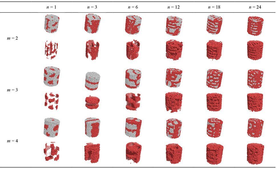
It is seen from Table 1 that the morphologies of lamella-forming (in the bulk) macromolecules (n = 3, m = 2–4) depend on the side chain length m. At m = 2 some of units B form a sort of a stripe or a central rod along the capillary axis, whereas the rest of units B concentrate in a thin layer near the capillary wall. For the longer side chains (m = 3, 4), the lamellar morphology stays basically intact except for some minor modifications, with the lamellae both parallel and normal to the cylinder axis being observed. In the former case, a central lamella of units B goes along the cylinder axis, whereas the rest of units B gather near the capillary walls (see Table 1, n = 3, m = 4). It is worth noting that in a series of independent calculations the parallel and perpendicular lamellae were observed with equal probabilities both for m = 3 and m = 4. Based on these calculations, we conclude that these structures are thermodynamically equivalent, so that lamellae take their orientations randomly.
The morphology of "mutually perpendicular lamellae" formed in the bulk by macromolecules with n = 6 transforms in a pore just into a mixture of parallel and normal lamellae, first appearing for n = 3. To summarize, for m = 2 a sort of parallel lamella is formed, for m = 3 a bicontinuous network appears, for m = 4 units B seem to form a sort of perforated lamella perpendicular to the pore axis.
A further increase of n (n ≥ 12) leads to the formation of structures that strongly resemble those in the bulk for the same values of m and n (see Figs. 2d,e and Table 1).
Now, let us turn to the results for the thinner capillaries (R = 20). The corresponding typical snapshots (with units B shown only) are presented in Table 2.
Table 2. Typical snapshots of the systems in the capillary (units B are only shown) at different values of m and n. H = 128, R = 20, εAB = 8
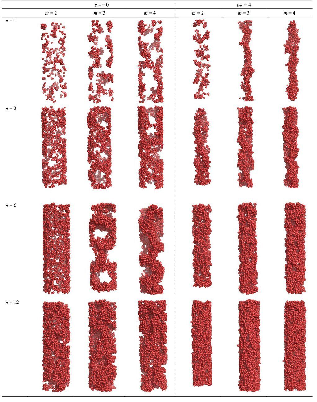
It can be seen from Table 2 that, for the nonselective pore wall (εBC = 0), most of side chain units B shift towards the wall and form a sort of a tube. On the surface of this tube, the units are distributed randomly for m = 2, n = 1–12, but with an increase of m they become correlated. Say, at n = 1 and m = 4, the units B gather in thin interweaving threads, and, at n = 6 and m = 4, they gather into a sort of spiral-like patterns on the capillary surface. The microstructures at n = 6 and m = 3 look like a set of rings formed by the units B and connected normally to each other. At n = 12, m = 3, the capillary surface is covered with a nonuniform layer of units B with the inhomogeneity scale being of an order of the capillary radius.
On the contrary, if units B are repelled from the wall, then, as is seen from Table 2, they are shifted towards the cylinder axis. Remarkably, the selective interactions with the pore wall can result in both appearance and disappearance of the spiral-like patterns (for example, cf. snapshots for n = 1 and n = 3 in Table 2).
Thus, the copolymer morphologies formed upon ordering under cylindrical confinement can be described essentially less definitely than those in the bulk, the ordering being deteriorating with reducing capillary radius. The problem is that, as was discussed in Refs. 39, 40, and 53, the systems under cylindrical confinement are a sort of one-dimensional systems and, therefore, they cannot undergo sharp phase transitions in virtue of the famous Landau theorem [54]. Therefore, in a capillary we can define only the distribution of "structural modes" rather than pure well-defined microscopic phases. To clarify this point, it is important to remind an analogy between the phase segregation for 1D Ising (helix-coil transition) model and the ordering under cylindrical confinement [40].
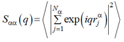
Indeed, by virtue of the Landau theorem [54], the ordered phase is formed as an alternating succession of the ordered and disordered areas (generally, of various lengths) rather than the only homogeneously ordered phase which fills the whole capillary. For simplicity, these areas are represented in Fig. 3 as black and white segments, respectively. (In fact, for the confined copolymers, one needs more colors to label the segments with all possible structure modes. However, even two-color picture would provide a sufficient basis for qualitative description).
![]()
Figure 3. Typical succession of the ordered (black) and disordered (white) capillary segments.
Hence, to describe the thermodynamics of the whole capillary, we are to evaluate its partition function similarly to that of 1D Ising model [55], which is presented in Appendix. In particular, it is shown in Appendix that the narrower the capillary, the less effective the cooperativity which determines the average length  of the ordered areas. Thus, if the capillary is narrow enough, then the length of the ordered area can be less than the longitudinal period L which characterizes the resulting structure mode. In this case, the finite size effects become strong enough to destroy the long ordering in the capillary. Just this effect, the strong radius-dependent ordering suppression in the narrow capillaries, we see in Tables 1 and 2.
Another way to evaluate the ordering in these only partially ordered systems quantitatively is the calculation of a correlation function, which would characterize such "structural modes". In the next Section we address this issue in more detail.
5. Cylindrical morphologies beyond the snapshot visual description: order parameter and structural modes
In this section we present the basics of the correlation function technique required to extract some quantitative information on the ordering of amphiphilic block copolymers under cylindrical confinement from the Monte Carlo simulation data. To begin with, it is worth mentioning that, as was shown earlier [39–41], the definition of an order parameter for flexible block copolymers is provided by the expansion coefficients of the composition spatial profile ψ (r) = φA (r) - φB (r) in eigen functions of the Laplace operator for the given type of confinement and boundary conditions.
In the bulk, the procedure corresponds just to the Fourier integral:
| (10) |
and the Fourier series (for nonperiodic and periodic inhomogeneities, respectively):
| (11) |
where summation is to be done over all vectors qi, which belong to the reciprocal lattice corresponding to the chosen crystal lattice. One can say, bearing in mind future generalization, that any bulk inhomogeneity is a sum of properly weighted elementary structural modes that are just plain harmonics characterized by their wave vector q:
 |
(12) |
For cylindrical geometry, representations (10) and (11) read [39, 40]:
 |
, (10a) |
 |
, (11a) |
where ρ = r/R is the reduced polar radius, Jm(x) is the Bessel coefficient [56] of order m, αm,n is the n-th member of the sequence of eigen values of the Bessel equation satisfying the imposed boundary condition (say,  or Jm(αn) = 0), and q is the longitudinal wave number, q = 2π/L where L is the longitudinal period. So, the elementary structural modes for cylindrical geometry can be defined as running
 |
(13a) |
or standing waves
 |
(13b) |
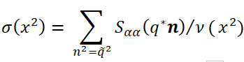
It should be noted that in Sections 5 and 6 the designations m and n are used only to characterize the symmetry of the structural modes that appear in Eqs. (10a), (11a) and (13), and they have nothing common with the architectural variables m and n that appear in the model of amphiphilic copolymer presented in Fig. 1. Remarkably, rigorous consideration based on representation (11a) enables one to prove that the shapes corresponding to the stable one- and double-stranded helices entwined around a rigid rod could exist also in the lamellar-forming block copolymers, provided that the surface field, confinement and overcooling are strong enough [40]. Another advantage of the rigorous analytical approach [40] is that it enables us to consider many seemingly complex shapes just as elementary structural modes (13), some of which are shown in Figs. 4–7, where the order parameter distributions corresponding to the simplest structural modes are visualized with normalization, which is convenient for the visualization procedure and is physically irrelevant. In other words, the colors in Figs. 4–7 indicate the relative ordering only (red and blue colors correspond to the minimal and maximal values of the order parameter, respectively; the numbers labeling the colors characterize qualitatively the relationship between the colors and the degree of segregation).
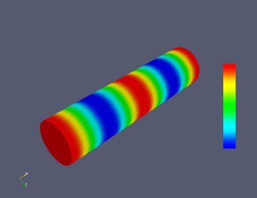
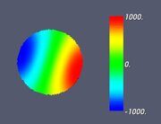
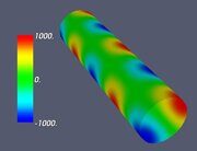
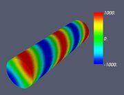
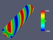
Figure 4. Classifying the microphase separated morphologies as the structural modes (13): longitudinally modulated morphology with Ψ = cos (4π z / L) (perpendicular lamella).
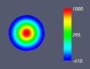
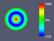
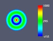
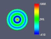
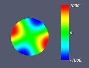
Figure 5. Classifying the microphase separated morphologies as the structural modes (13): radially modulated (coaxial) morphologies corresponding to Ψ = J (α0,n ρ) with n = 1, 2, 3, 4 (from left to right, respectively). The coaxial morphologies with the higher numbers of the blue and yellow-green circles would correspond to the higher values of n.
 |
 |
 |
 |
| a | b | c | d |
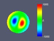
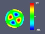
Figure 6. Classifying the microphase separated morphologies as the structural modes (13): morphologies with angular and radial modulation corresponding to Ψ = J (αm,n ρ) cos (mφ) . (a): m = 1, n = 1 (Janus cylinder); (b) m = 1, n = 2 (hidden Janus cylinder); (c) m = 2, n = 1 (double Janus cylinder); (d) m = 2, n = 2 (double hidden Janus cylinder).
 |
 |
 |
 |
| a | b | c | d |
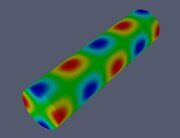
Figure 7. Classifying the microphase separated morphologies as the structural modes (13): fully modulated morphologies. (a) Janus helix, (b) alternating Janus cylinder, (c) double Janus helix, (d) alternating double Janus cylinder. The eigen functions (13) corresponding to these morphologies are as follows: (a) single helix Ψ = J1 (α1,1 ρ) cos (φ - 4π z / L), (b) alternating Janus cylinder Ψ = J1 (α1,1 ρ) cos (φ) cos (4π z / L) (c) double helix Ψ = J2 (α2,1 ρ) cos (2φ - 4π z / L), (d) alternating double Janus cylinder Ψ = J2 (α2,1 ρ) cos (2φ) cos (4π z / L).
Let us make some comments here. First, some of the images shown in Figs. 4–7 were already presented earlier in various computer simulation and SCFT studies (e.g., the images very close to those shown in Fig. 4 can be found in Refs. 20, 27 and 28). What is new is that all such shapes are just simple structural modes (13) naturally related to the very fact of confinement in cylindric geometry. Second, it is informative to compare the snapshots shown in Table 2 and the alternating double Janus cylinder presented in Fig. 7d. Obviously, their symmetries are the same. (Indeed, the holes, which are most clearly seen in the snapshot shown in Table 2 for m = 3, n = 6 and εBC = 0, correspond to the maximal lack of units B or, in other words, correspond to the blue spots on the last images in Fig. 7d).
It is worth noting here that the very existence of a parallel between strongly segregated morphologies with εAB = 8 shown in Table 2 and weakly segregated one depicted in Fig. 7d is far from being obvious. Nevertheless, one can find several reasons for this. First, even though the local properties (say, the width of the interdomain surfaces) may be rather different in the strong and weak segregation theories, the proper global properties (say, the general symmetry of the phases formed and a general outlook of the phase diagram) are rather similar. (For segregation theories for diblock copolymers, see Refs. 45 (weak), 57, 58 (intermediate) and 59 (strong). For segregation theories for ternary ABC block copolymers, see Refs. 12 (weak) and 13, 60, and 61 (intermediate).) Second, as it has been shown recently [62], the formation of inhomogeneous morphologies in the confined volume requires much bigger incompatibility between the copolymer units than in the bulk, which means that the case εAB = 8 may correspond to weak or intermediate segregation. We suppose to return to this issue in more detail elsewhere.
To conclude, we introduce the sectoral number density of the units of the i-th sort, which lumps together the patterns with different radial behaviors.
 , (14)
where  is the conventional number density of the units of the i-th sort as a function of the cylindrical coordinates, r (ni) , φ (ni) , and z (ni) being radius-vector, axial coordinate z and polar angle j of the n-th particle of the i-th sort, respectively. Summation runs over all Ni particles of this sort.
Both the advantage and deficiency of the sectoral density (14) is that its Fourier transform which we call spectral sectoral density (SSD)
 |
(15) |
enables us to split contributions of the patterns with different angular and longitudinal symmetry, but lumps together the patterns with different radial behaviors. Say, the morphology shown in Fig. 3 contributes into  with a certain finite value of q, whereas the morphologies shown in Fig. 4 all contribute into
  only. Morphologies shown in Figs. 6a and 6b and Figs. 7a and 7b contribute into and . At last, the morphologies shown in Figs. 6c and 6d and Figs. 7c and 7d contribute into functions
  and
and  , respectively.
6. Correlation functions technique and morphologies of the amphiphilic diblock copolymers under cylindrical confinement
The above considerations suggest that the computer simulation data (momentary and averaged snapshots, etc.) can be interpreted in terms of the structural modes (13) either. However, the way of extraction of the desired structural information from the data of simulations is far from being obvious. Indeed, the momentary snapshots can be not too representative, whereas the averaged ones can be too smeared. Besides, to extract the radial modes, we need the actual form of the boundary conditions that determine the sequence αm,n of the eigen values. But the latter can not be directly related to the microscopic copolymer model used under computer simulations. (The situation here resembles that with the relationship between theoretical χ-parameters and microscopic interaction potentials.) At last, some structures can correspond to superpositions of the structural modes rather than to the pure ones.
So, to forget the radial behavior, we make use of the sectoral densities (14) and instead of dealing with the averaged morphology (1-point order parameter) we consider sectoral correlation function (2-point order parameter)
 |
(16) |
that describes correlations between the total densities of the sectors, which are, as shown in Fig. 8, at the distance z = z2 - z1 along the cylinder axis and are rotated at the angle Δφ = φ2 - φ1 from each other.
The Fourier transform of the function (16) we call sectoral structure factor (SSF) is
 |
(17) |
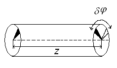
Figure 8. Schematic representation of the correlation function (16).
Here  is defined by Eq (15), the bar and brackets mean complex conjugation and thermodynamic averaging, respectively, and the longitudinal wave number runs the values q = 2πl/H, l = 1, 2…, ∞. Obviously, both expressions (15) and (17) can be easily evaluated numerically using the simulation data.
More specifically, we considered the normalized SSF for the BB units:
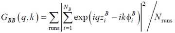 |
, (18) |
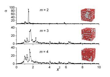
where Nruns is the number of runs. It was calculated every 102 steps in the course of 106 consecutive Monte Carlo steps and next averaged over time and seven independent runs. The results are plotted in Figs. 9–11 for k = 0, 1, 2 and the most representative compositions of the amphiphilic block (see Table 2). The log-log scales are used to see the correlation behavior on all accessible scales.

Figure 9. Correlation functions GBB(q,k) for n = 1 and m = 2 (a), m = 3 (b), and m = 4 (c). H = 128, R = 20, εBC = 0, εAB = 8. The filled squares (■), circles (·) and triangles (▲) display the data for k = 0, k = 1, and k = 2, respectively. The dashed lines are guides for eyes.
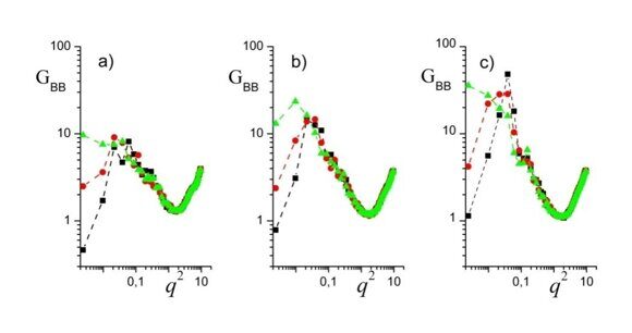
Figure 10. Correlation functions GBB(q, k) for n = 3 and m = 2 (a), m = 3 (b), and m = 4 (c). H = 128, R = 20, εBC = 0, εAB = 8. The filled squares (■), circles (·) and triangles (▲) display the data for k = 0, k = 1, and k = 2, respectively. The dashed lines are the guides for eyes.
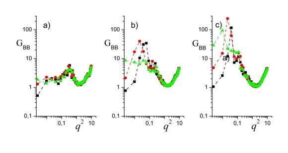
Figure 11. Correlation functions GBB(q, k) for n = 6 and m = 2 (a), m = 3 (b), and m = 4 (c). H = 128, R = 20, εBC = 0, εAB = 8. The filled squares (■), circles (·) and triangles (▲) display the data for k = 0, k = 1, and k = 2, respectively. The dashed lines are the guides for eyes.
First, most (but not all!) of the plots reveal a small-angle peak due to the correlation hole effect [44], which is typical for block copolymer melts upon ordering. The peak indicates that the correlation function Sjj(0,0,z,0) is a decaying function oscillating with the period of L* = 2π/q*, where q* is the location of the peak. Next, all quantities under study reveal an intermediate-q descending branch G ~ 1 / q2, which is characteristic of homopolymer mixtures. It corresponds to the behavior on the intermediate scales, which are already much less than L* (on these scales the blocks "forget" that they are connected), but still big compared to the scale of the inter-unit potential a. At last, all the plots reveal practically the same high-q ascending branch. It is quite natural, since the branch corresponds to an increase of the short-range correlations in dense liquids on scales of the order of a. Now, let us consider in more detail the distinctions between different correlations.
It can be seen from Fig. 9 that the height of the small-angle peak increases with an increase of the amphiphilic tail. One more informative feature of the plots presented in Fig. 9 is that the low-q correlations increase as the order k, which characterizes the angle correlations, grows:
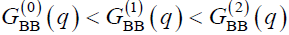 (19)
(19)
It means that the angle modulation corresponding to both Janus (Figs. 6a,b and Figs. 7a,b) and double Janus (Figs. 6c,d and Figs. 7c,d) behavior is more pronounced for the higher overall longitudinal scale. At last, unlike the effective structure factor presented in Fig. 2, SSF plotted in Fig. 9 reveals no secondary peaks, which indicates that no genuine 1D ordering occurs along the cylinder axes.§ Thus, even though for n = 1 and m = 4 our system in the bulk is just an asymmetric linear A–B block copolymer forming well-ordered morphologies, the cylindrical confinement reduces this ordering only to some order parameter oscillations that decay along the cylinder axes and have a period corresponding to the bulk lamellar period. (We have already noticed the ordering suppression by cylindrical confinement in Section 4, when we compared the snapshots from Table 1 and Table 2.).
Similar features can be seen in Figs. 10 and 11. Here we also do not see any secondary peak§, and inequalities (19) hold in the low-q region. The latter feature is consistent with our earlier theoretical results [39, 40], according to which GBB(q,k2) can be obtained from GBB(q,k1) with k2 > k1 via a shift of the entire plot to the left. Sometimes such shifts to the left are so big that the maximum on the curve GBB(q,2) moves to an unphysical region q2 < 0 and, thus, disappears (see Figs. 10a,c and 11a,b). Remarkably, there is a strong correspondence between the systems that exhibit such a behavior and fluctuate strongly enough (see Figs. 10c and 11b) and those, for which the characteristic snapshots are the so-called catenoid-cylinders (Table 2, n = 3, m = 4 and n = 6, m = 3). More precisely, even though there are no pure structural modes (no pure lamellae, no pure Januses, etc.) under cylindrical confinement as was explained above, there are fluctuating structural excitations whose correlations are presented in Figs. 9–11. And the systems, where the double Janus-like excitations are stronger correlated, are just those systems where human eyes are inclined to detect the catenoid-cylinder snapshots. Such a correspondence is no surprise, if we recall the resemblance between catenoid-cylinders and double Janus structural modes (Fig. 7).
7. Conclusions
To summarize the result presented, in this work we studied the phase and morphological behavior of amphiphilic block copolymers using the Monte Carlo simulations in cubic and cylindrical cells for various temperatures and block copolymer architectures. The data obtained were analyzed both visually (via selecting typical snapshots) and quantitatively (using the correlation functions technique). For the morphologies of block copolymers under cylindrical confinement, the symmetry classification of the structural modes was discussed in detail and a special (sectoral) structure factor was introduced to characterize these morphologies quantitatively (for the first time for amphiphilic copolymers).
In the bulk, the amphiphilic copolymers under consideration were found to have an extra (compared to the conventional diblock copolymers) tendency to form bi-continuous morphologies. The morphologies evolving upon changing of the amphiphilic block composition were identified via the structure factor analysis. Under cylindrical confinement, a strong effect of the ordering suppression with a decrease of the capillary radius was found both analytically and via computer simulations. As a result, no genuine long ordering along the cylinder axes occurred. However, on finite scales, the amphiphilic copolymers with the composition, which corresponds to the bi-continuous morphologies in the bulk, under cylindrical confinement revealed a short-range order locally resembling Janus and double Janus cylinder morphologies.
Appendix. 1D Ising model and ordering under cylindrical confinement
To evaluate the partition function Z(L) of the system and to extract the basic features of ordering under cylindrical confinement from the latter, let us start with writing down Z(L) in the following form
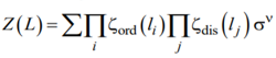 |
, (A1) |
where L is the total length of the capillary filled with the copolymer,
 |
, (A2) |
are the partition functions to be assigned to a homogeneous segments of the length l in the α-th state (α = ord, disord), and fα is the specific (per unit length along the capillary axes) free energy of the a-th phase. Obviously,  , R and
  being the capillary radius and specific (per unit volume) free energy of the a-th phase, respectively. {li} and {lj} are sets of the lengths of the disordered and ordered segments, respectively. s is the factor to be assigned to the order-disorder interface. From general considerations, σ = σ0 exp( finter / T), where σ0 is a phenomenological constant of the dimensionality [L]–1 and
 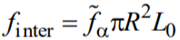 is an extra free energy per the order-disorder interface, L0 being the characteristic width of the order-disorder interface. At last, n is the total number of the order-disorder interfaces. Summation in (A1) is over all permutations of the black and white segments with different lengths.
By analogy with the coil-helix transition [55], the Laplace transform ![]() reads:
reads:
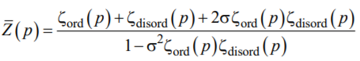 |
, (A3) |
where
 |
(A4) |
with Δf = ford – fdisord. The partition function Z(L) is the inverse Laplace transform [63]:
 |
(A5) |
and, therefore, it is determined by the poles of function (A3).
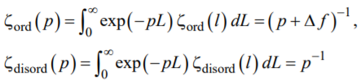
It follows from Eqs. (A1)–(A5) that the length fraction φord of the ordered segments and the average length  of the ordered segments are continuous functions
 |
(A6) |
where ![]() is the relevant pole of the inverse Laplace transform (A3) and u = Δf (2σ). Obviously, i) φord > 0.5 for u < 0 and φord < 0.5 for u > 0. and ii) both φord and lord tend to infinity when the parameter u tends to infinity. Taking into account the above definition of s, we see that when R diminishes, the ordering deteriorates and, finally, disappears in accordance with our results discussed in Section 4.
is the relevant pole of the inverse Laplace transform (A3) and u = Δf (2σ). Obviously, i) φord > 0.5 for u < 0 and φord < 0.5 for u > 0. and ii) both φord and lord tend to infinity when the parameter u tends to infinity. Taking into account the above definition of s, we see that when R diminishes, the ordering deteriorates and, finally, disappears in accordance with our results discussed in Section 4.
Acknowledgements
This work was supported by the Ministry of Science and Higher Education of the Russian Federation. The research was carried out using the equipment of the shared research facilities of HPC computing resources at Lomonosov Moscow State University [64].
References and notes
§ There are, though, some indications of the irregular secondary peaks in Figs. 9a, 10a, and 11a,b,c. However, we are inclined to assign these peaks to scarcity of our data to provide their sufficient statistical averaging.
- F. S. Bates, G. H. Fredrickson, Annu. Rev. Phys. Chem., 1990, 41, 525–557. DOI: 10.1146/annurev.pc.41.100190.002521
- I. Ya. Erukhimovich, A. R. Khokhlov, Polym. Sci., Ser. A, 1993, 35, 1522–1531.
- K. Binder, Adv. Polym. Sci., 1994, 112, 181–299. DOI: 10.1007/BFb0017984
- F. S. Bates, G. H. Fredrickson, Phys. Today, 1999, 52, 32–38. DOI: 10.1063/1.882522
- Supramolecular Polymers, A. Ciferri (Ed.), New York, Basel, Marcell Dekker, 2000.
- Block Copolymers in Nanoscience, M. Lazzari, G. Liu, S. Lecommandoux (Eds.), Weinheim, Wiley, 2006.
- Nanostructured Soft Matter: Experiment, Theory, Simulation and Perspectives, NanoScience and Technology, A. V. Zvelindovsky (Ed.), Dordrecht, Springer, 2007.
- C. A. Tyler, D. C. Morse, Phys. Rev. Lett., 2005, 94, 208302. DOI: 10.1103/PhysRevLett.94.208302
- A. Ranjan, D. C. Morse, Phys. Rev. E, 2006, 74, 011803. DOI: 10.1103/PhysRevE.74.011803
- T. H. Epps, E. W. Cochran, C. M. Hardy, T. S. Bailey, R. S. Waletzko, F. S. Bates, Macromolecules, 2004, 37, 7085–7088. DOI: 10.1021/ma0493426
- J. Chatterjee, S. Jain, F. S. Bates, Macromolecules, 2007, 40, 2882–2896. DOI: 10.1021/ma062249s
- I. Y. Erukhimovich, Eur. Phys. J. E: Soft Matter Biol. Phys., 2005, 18, 383–406. DOI: 10.1140/epje/e2005-00054-5
- J. Qin, F. S. Bates, D. C. Morse, Macromolecules, 2010, 43, 5128–5136. DOI: 10.1021/ma100400q
- H. Xiang, K. Shin, T. Kim, S. I. Moon, T. J. McCarthy, T. P. Russell, Macromolecules, 2004, 37, 5660–5664. DOI: 10.1021/ma049299m
- Y. Sun, M. Steinhart, D. Zschech, R. Adhikari, G. H. Michler, U. Gösele, Macromol. Rapid Commun., 2005, 26, 369–375. DOI: 10.1002/marc.200400545
- H. Xiang, K. Shin, T. Kim, S. I. Moon, T. J. McCarthy, T. P. Russell, Macromolecules, 2005, 38, 1055–1056. DOI: 10.1021/ma0476036
- H. Xiang, K. Shin, T. Kim, S. Moon, T. J. McCarthy, T. P. Russell, J. Polym. Sci., Part B: Polym. Phys., 2005, 43, 3377–3383. DOI: 10.1002/polb.20641
- P. Dobriyal, H. Xiang, M. Kazuyuki, J.-T. Chen, H. Jinnai, T. P. Russell, Macromolecules, 2009, 42, 9082–9088. DOI: 10.1021/ma901730a
- X. He, M. Song, H. Liang, C. Pan, J. Chem. Phys., 2001, 114, 10510–10513. DOI: 10.1063/1.1372189
- G. J. A. Sevink, A. V. Zvelindovsky, J. G. E. M. Fraaije, H. P. Huinink, J. Chem. Phys., 2001, 115, 8226–8230. DOI: 10.1063/1.1403437
- P. Chen, X. He, H. Liang, J. Chem. Phys., 2006, 124, 104906. DOI: 10.1063/1.2178802
- J. Feng, E. Ruckenstein, Macromolecules, 2006, 39, 4899–4906. DOI: 10.1021/ma0605954
- Q. Wang, J. Chem. Phys., 2007, 126, 024903. DOI: 10.1063/1.2406078
- J. Feng, H. Liu, Y. Hu, Macromol. Theory Simul., 2006, 15, 674–685. DOI: 10.1002/mats.200600042
- B. Yu, P. Sun, T. Chen, Q. Jin, D. Ding, B. Li, A.-C. Shi, J. Chem. Phys., 2007, 127, 114906. DOI: 10.1063/1.2768920
- M. Ma, E. L. Thomas, G. C. Rutledge, B. Yu, B. Li, Q. Jin, D. Ding, A.-C. Shi, Мacromolecules, 2010, 43, 3061–3071. DOI: 10.1021/ma9022586
- W. Li, R. A. Wickham, R. A. Garbary, Macromolecules, 2006, 39, 806–811. DOI: 10.1021/ma052151y
- W. Li, R. A. Wickham, Macromolecules, 2009, 42, 7530–7536. DOI: 10.1021/ma900667w
- A.-C. Shi, B. Li, Soft Matter, 2013, 9, 1398–1413. DOI: 10.1039/C2SM27031E
- A. R. Khokhlov, P. G. Khalatur, Chem. Phys. Lett., 2008, 461, 58–63. DOI: 10.1016/j.cplett.2008.06.054
- A. A. Glagoleva, V. V. Vasilevskaya, A. R. Khokhlov, Polym. Sci., Ser. A, 2010, 52, 182–190. DOI: 10.1134/S0965545X10020124
- A. Glagoleva, I. Erukhimovich, V. Vasilevskaya, Macromol. Theory Simul., 2013, 22, 31–35. DOI: 10.1002/mats.201200056
- Yu. A. Kriksin, P. G. Khalatur, I. Ya. Erukhimovich, G. ten Brinke, A. R. Khokhlov, Soft Matter, 2009, 5, 2896–2904, DOI: 10.1039/B905923G
- S. Basu, D. R. Vutukuri, S. Shyamroy, B. S. Sandanaraj, S. Thayumanavan, J. Am. Chem. Soc., 2004, 126, 9890–9891. DOI: 10.1021/ja047816a
- V. V. Vasilevskaya, P. G. Khalatur, A. R. Khokhlov, Macromolecules, 2003, 36, 10103–10111. DOI: 10.1021/ma0350563
- V. V. Vasilevskaya, A. A. Klochkov, A. A. Lazutin, P. G. Khalatur, A. R. Khokhlov, Macromolecules, 2004, 37, 5444–5460. DOI: 10.1021/ma0359741
- V. V. Vasilevskaya, V. A. Ermilov, Polym. Sci., Ser. A, 2011, 53, 846–866. DOI: 10.1134/S0965545X11090148
- T. S. Kale, A. Klaikherd, B. Popere, S. Thayumanavan, Langmuir, 2009, 25, 9660–9670. DOI: 10.1021/la900734d
- I. Erukhimovich, P. E. Theodorakis, W. Paul, K. Binder, J. Chem. Phys., 2011, 134, 054906. DOI: 10.1063/1.3537978
- I. Erukhimovich, A. Johner, Europhys. Lett., 2007, 79, 56004. DOI: 10.1209/0295-5075/79/56004
- B. Miao, D. Yan, C. C. Han, A.-C. Shi, J. Chem. Phys., 2006, 124, 144902. DOI: 10.1063/1.2187492
- I. Carmesin, K. Kremer, Macromolecules, 1988, 21, 2819–2823. DOI: 10.1021/ma00187a030
- K. Binder, W. Paul, J. Polym. Sci., Part B: Polym. Phys., 1997, 35, 1–31. DOI: 10.1002/(SICI)1099-0488(19970115)35:1<1::AID-POLB1>3.0.CO;2-#
- P.-G. de Gennes, Scaling Concepts in Polymer Physics, Cornell Univ. Press, 1979.
- L. Leibler, Macromolecules, 1980, 13, 1602–1617. DOI: 10.1021/ma60078a047
- L. D. Landau, E. M. Lifshitz, Electrodynamics of Continuous Media, Oxford, New York, Beijing, Frankfurt, Pergamon Press, 1984.
- P. Garstecki, R. Hołyst, J. Chem. Phys., 2001, 115, 1095–1099. DOI: 10.1063/1.1379326
- P. Garstecki, R. Hołyst, Macromolecules, 2003, 36, 9191–9198. DOI: 10.1021/ma0212590
- S. Lee, M. J. Bluemle, F. S. Bates, Science, 2010, 330, 349–353. DOI: 10.1126/science.1195552
- J. Zhang, F. S. Bates, J. Am. Chem. Soc., 2012, 134, 7636–7639. DOI: 10.1021/ja301770v
- N. Xie, W. Li, F. Qiu, A.-C. Shi, ACS Macro Lett., 2014, 3, 906–910. DOI: 10.1021/mz500445v
- M. Liu, W. Li, F. Qiu, A.-C. Shi, Soft Matter, 2016, 12, 6412–6421. DOI: 10.1039/C6SM00798H
- H.-P. Hsu, W. Paul, K. Binder, Europhys. Lett., 2006, 76, 526–532. DOI: 10.1209/epl/i2006-10276-4
- L. D. Landau, E. M. Lifshitz, Statistical Physics, Part 1, 3rd ed., Pergamon Press, 1980.
- A. Yu. Grosberg, A. R. Khokhlov, Statistical Physics of Macromolecules, New York, AIP Press, 1994.
- G. N. Watson, A Treatise on the Theory of Bessel Functions, Second Edition, Cambridge, Univ. Press, 1995.
- M. W. Matsen, M. Schick, Phys. Rev. Lett., 1994, 72, 2660–2663. DOI: 10.1103/PhysRevLett.72.2660
- M. Matsen, F. S. Bates, Macromolecules, 1996, 29, 1091–1098. DOI: 10.1021/ma951138i
- A. N. Semenov, Sov. Phys. JETP, 1985, 61, 733–742.
- Yu. A. Kriksin, I. Ya. Erukhimovich, P. G. Khalatur, Yu. G. Smirnova, G. ten Brinke, J. Chem. Phys., 2008, 128, 244903. DOI: 10.1063/1.2937138
- I. Erukhimovich, Y. Kriksin, G. ten Brinke, Soft Matter, 2012, 8, 2159–2169. DOI: 10.1039/c1sm06688a
- I. Erukhimovich, Polym. Sci., Ser. C, 2018, 60, 49–55. DOI: 10.1134/S1811238218020066
- G. Doetsch, Introduction to the Theory and Application of the Laplace Transformation, Berlin, Heidelberg, Springer, 1974.
- V. Sadovnichy, A. Tikhonravov, V. Voevodin, V. Opanasenko, in: Contemporary High Performance Computing: From Petascale toward Exascale, Boca Raton, CRC Press, 2013, pp. 283–307.