2021 Volume 4 Issue 5

Open Access

INEOS OPEN, 2021, 4 (5), 154–175  Journal of Nesmeyanov Institute of Organoelement Compounds of the Russian Academy of Sciences Download PDF Electronic supplementary information DOI: 10.32931/io2125r

Modern Criteria of Aromaticity for Organometallic Compounds

Abstract

Aromaticity as one of the most important fundamental concepts in chemistry is an effect of cyclic electron delocalization, which is very multifaceted and difficult to measure. To define the aromaticity degree as a quantitative characteristic, the aromaticity indices are used that can be divided into energetic, structural, electronic, magnetic, and optical. The aromaticity effect went far beyond the class of π-conjugated hydrocarbons a long time ago; therefore, this review critically examines the most important and modern criteria of aromaticity which are universal in the system choice and have been applied to organometallic compounds.

Key words: electron delocalization, aromaticity, modern criteria of aromaticity, organometallic compounds.

 

Abbreviations

ACID – anisotropy of the induced current density
AdNDP – adaptive natural density partitioning
ASE – aromatic stabilization energy
BAC – bond alternating coefficient
BLW – block-localized wave function
CDA – current density analysis
CMO – canonical molecular orbital
СTED – corrected total electron density
CTOCD – continuous transformation of the origin of the current density
DRE – Dewar resonance energy
DI – delocalization index
EDA – energy decomposition analysis
EDDB – electron density of delocalized bonds
FLU – aromatic fluctuation index
FBO – fuzzy bond order
GIAO – gauge-including atomic orbital
GIMIC – gauge-including magnetically induced currents
HOMA – harmonic oscillator model of aromaticity
HRE – Hückel resonance energy
ICSS – iso-chemical shielding surface
IRCS – induced ring current strength
ISE – isomerization stabilization energy
MICD – magnetically induced current density
NICS – nucleus-independent chemical shift
NBO – natural bond orbital
NODB – natural orbitals of delocalized bonds
PDI – para-delocalization index
RE – resonance energy
QTAIM – quantum theory "Atoms in molecules"

1. Introduction

Aromaticity (from Greek aroma, genitive aromatos—sweet smell) is one of the fundamental concepts [1] in modern chemistry along with the notions of a charge, chemical bond, acidity, basicity, etc. It is hard to find another concept in the current chemical theory that would feature such a high generality degree, play such an important role for systematization, and, at the same time, be so vague and ambiguous.

Aromaticity is a phenomenon of electron delocalization in closed cycles or three-dimensional cages that leads to a reduction in energy and numerous unusual chemical and physical properties. These properties include a propensity for equalization of bond lengths, chemical behavior with the structure retention, and characteristic magnetic and spectroscopic properties [2].

Aromaticity is considered a multidimensional system property that is easy to recognize but difficult to measure directly. The aromaticity degree, which represents a quantitative characteristic, is defined for one or another system by the application of aromaticity criteria, both the experimental and theoretical ones. Although since the mid-2000s the aromaticity concept can be considered established, it has been continuously developing along with the molecular electronic structure theory [1].

Several special issues of the leading chemical review journals published in 2001 [3], 2005 [4], and 2015 [5], as well as a special book issued in 2021 [1] are devoted to the aromaticity concept. They generalize the most important results of investigations on the aromatic molecules.

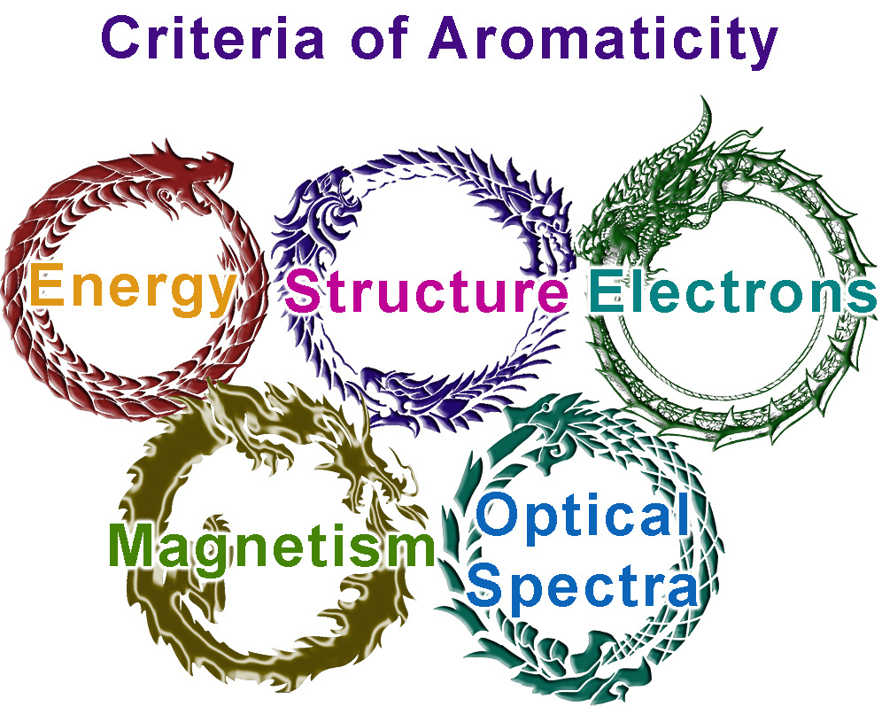
The aromaticity as a cyclic conjugation can be of various types (Fig. 1, Table 1) which differ in the conjugation mechanism, topology, and spatial structure. Along with the most popular Hückel π-aromaticity [6], of particular importance is the Möbius aromaticity for non-planar (twisted) annulenes [7]. The stable electronic configuration of the latter consists of 4n π‑electrons, whereas for planar annulenes, this is the antiaromatic configuration [8]. The complementary approaches of the Möbius and Hückel aromaticity allow for an exhaustive explanation of the aromatic or antiaromatic characters of different annulenes and heterocycles, as well as the direction of sigmatropic rearrangements and the stereochemistry of electrocyclic reactions [9]. The aromaticity notion has gone far beyond the π‑delocalization phenomenon. Thus, the aromaticity can be realized through the conjugation of σ- [10], d- [11, 12], and f-orbitals [13] between each other and with π-orbitals, and can be partial, double [14], triple [15], in-plane [16], and three-dimensional [17–19] (Fig. 1). A combination of the Möbius aromaticity with a phase inversion owing to d-orbitals is classified as the Craig aromaticity [11]. The phenomenon of homoaromaticity arises in the case when the conjugating centers are interrupted by a saturated unit, for example, a CH₂ group or another ordinary unit bearing a heteroatom [20]. The cyclic delocalization of σ-electrons is called σ-aromaticity, which takes place, for example, in cyclopropane [10c] and hexahalogen-substituted benzenes [21]. Recently, several new types of aromaticity have been revealed, among which of particular note are δ-aromaticity [22], f‑orbital [15], and adaptive aromaticity [23]. The latter represents a combination of the Hückel π-aromaticity in the ground state of a metallacycle and the Baird aromaticity in the excited state [24]. A peculiar type of aromaticity that involves a metal atom is comprised by the delocalization owing to the conjugation of multicenter M–C dative bonds [25, 26], which can be abbreviated to mc‑M–C-aromaticity. Importantly, the electron counting rules 4n + 2 or 4n are universal and remain valid for many types of aromaticity (Table 1).

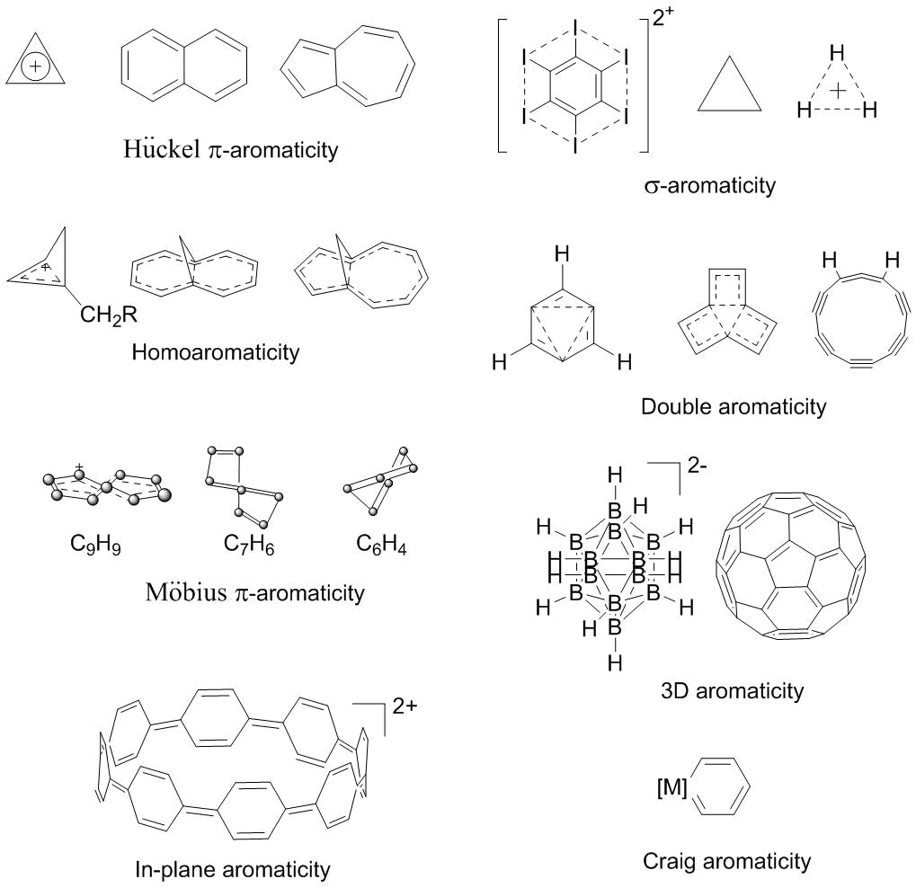
Figure 1. Examples of different types of aromaticity.

Table 1. Known types of aromaticity and the corresponding electron counting rules

Year	Author	Aromaticity type	Ref.
1931	E. Hückel	4n + 2 aromaticity rule for π-electrons in cyclic systems		[6]
1938	M. G. Evans, E. Warhurst	Aromaticity of transition states of pericyclic reactions		[9]
1958	D. P. Craig	Craig aromaticity with the inverse phase owing to the consideration of d-orbitals (4n)		[11]
1959	S. Winstein	Homoaromaticity (4n + 2)		[20]
1964	E. Heilbronner	Möbius aromaticity (4n) in twisted annulenes		[7]
1965	R. Breslow	Antiaromaticity (4n or 4n + 2)		[8]
1971	K. Wade	2n + 2 rule for cage electrons in closo-boranes		[18]
1972	D. M. P. Mingos	4n + 2 rule for valence electrons in closo-boranes		[19]
1972	N. C. Baird	Triplet aromaticity (4n)		[24]
1978	J Aihara	Three-dimensional aromaticity		[17]
1979	M. J. S. Dewar	σ-Aromaticity (4n + 2)		[10]
1979	P. v. R. Schleyer	Double aromaticity		[14]
1979	D. L. Torn, R. Hoffman	Aromaticity of metallabenzenes		[27]
1982	P. v. R. Schleyer, E. D. Jemmis	Generalization of the 4n + 2 electron counting rule for pyramidal molecules		[28]
1986	A. B. McEwen, P. v. R. Schleyer	In-plane aromaticity (4n + 2)		[16]
2000	A. Hirsh	2(n + 1)2 rule for spherical aromaticity		[29]
2005	P. v. R. Schleyer	d-Orbital aromaticity		[12]
2007	A. I. Boldyrev	δ-Aromaticity		[22]
2007	B. B. Averkiev, A. I. Boldyrev	Triple (σ-, π-, and δ-) aromaticity		[15]
2008	A. C. Tsipis	f-Orbital aromaticity		[13]
2011	J. Poater, M. Sola	Spherical aromaticity with an open electron shell (2n2 + 2n + 1)		[30]
2013	R. W. A. Havenith	Aromaticity rule for disc-like molecules		[31]
2014	M. T. Nguyen	Cylindrical aromaticity		[32]
2015	B. Zhao, J. Li	Cubic aromaticity (6n + 2)		[33]
2018	J. Zhu	Adaptive aromaticity (4n or 4n + 2)		[23]
2021	R. R. Aysin	mc-M–C-aromaticity (4n + 2)		[25, 26]

2. Aromaticity criteria

To define the presence or absence of aromaticity in a particular compound as well as to estimate its degree, many physical properties are used as criteria that are characteristic of aromatic compounds. It is important to note that all the suggested criteria, first of all, confirm the aromatic character of an ideal aromatic molecule of benzene, and the parameter values for it are taken as a reference point. Some of these properties are applicable to any system, other properties can be used only for specific systems. A great variety of criteria stems from the fact that the properties of aromatic molecules deviate from the additive schemes. The main aromaticity criteria generally accepted in modern literature [1, 34] are as follows.

1. The energetic criteria comprise an increase in the stability of aromatic compounds compared to the non-aromatic analogs [35, 36].

2. The electronic criteria include the electron counting rules, the criteria based on bond orders, the localization and delocalization of orbitals, and the electron density distribution [37–39].

3. The structural criteria reflect the propensity of bond lengths in aromatic compounds for equalization (multiple bonds elongate and single bonds shorten relative to the bonds in non-aromatic analogs) [34, 40].

4. The magnetic criteria imply the appearance of ring currents upon application of an external magnetic field, which lead to an increase in the magnetic susceptibility, its anisotropy, and the specific values of chemical shifts in the NMR spectra [41–46].

5. The optical criteria include the shifts of absorption bands in the UV-vis spectra [47], a decrease in the vibration frequencies [48], and growth in the intensity of the Raman lines according to the theory of P. P. Shorygin [49].

2.1. Energetic criteria

The energetic criteria are based on the fact that the presence of aromaticity leads to an increase in the system stability, which violates the energy additivity. This was called stabilization energy (SE).

The first and most important method for measuring the stabilization energy of an aromatic compound is the calculation of the heat of combustion [50]. It is well known that the heat of combustion for saturated and non-aromatic hydrocarbons (HCs) is an additive value and can be calculated from the energies of separate bonds in hydrocarbons.

The formation enthalpy of benzene calculated from the experimental data using combustion reaction (1) is 1054.1 kcal/mol, while that calculated from the empirical values of the bond energies (С–H, C–C, and C=C) according to an additive scheme composes 1014.6 kcal/mol. The difference in 39.5 kcal/mol between the values of the experimental and calculated energies is called the resonance energy (RE). The analogous calculation using the heat of hydrogenation gives for benzene the RE value equal to 36.4 kcal/mol.

CxHy + (x+y/4) O2 = xCO2 + y/2 H2O      DHcomb(CxHy)

(1)

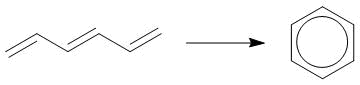
Scheme 1 presents the methods for measuring and calculating different stabilization energies based on isodesmic and homodesmic reactions (2)–(6). These and analogous reactions are widely used [35]. The calculation by equations (2) and (3) is called the resonance energies (REs), which characterize all the conjugation and aromaticity effects. The heats of reactions (4)–(6) are called the aromatic stabilization energies (ASE). Reactions (4)–(6) allow for estimating the additional stabilization only owing to the cyclic conjugation. The values of the ASE and RE are of particular importance for simple hydrocarbon systems since their calculation can be carried out based on the experimental heats of formation or combustion.

Scheme 1. Reactions for estimating the aromatic stabilization energy (ASE) and resonance energy (RE) on the example of a benzene molecule.

It is obvious that the main disadvantage of the above-mentioned energetic criteria is the dependence of the resulting value on the calculation scheme in use. The analysis of the ASE value by the reactions analogous to (4)–(6) for different five-membered rings bearing π-electrons showed that the application of non-cyclic model compounds provides unsatisfactory results since the ring strain is not taken into account. Therefore, only cyclic model compounds were suggested for the ASE calculations [51]. However, even in this case, there are still some drawbacks associated with the possible underestimation of the effect of ring strain, changes in the hybridization on passing from a model to the molecule under investigation, and the interaction of substituents with lone pairs. According to P. v. R. Schleyer, the most accurate scheme is the calculation by reaction (6). This equation was adopted for acenes, five- and six-membered heterocycles; the resulting ASE values are in good agreement with other data [35, 51–54].

A large group of RE evaluation approaches is based on the calculation of molecular orbital energies. Historically, the important approaches were those suggested by Hückel [35] and Dewar [55]. The Hückel resonance energy (HRE) for HCs is calculated by the Hückel method according to the following equation:

HRE = Eπ – n Eπ(CH2=CH2)

(7)

The HRE is a difference between the energies of π-orbitals of the system under consideration E_π and the energy of ethylene π-orbitals E_π(CH₂=CH₂) multiplied by the number of double bonds in the ring n. The Dewar resonance energy (DRE) takes into account a linear conjugation of double bonds, i.e., the DRE is equal to a difference in the energies of π-orbitals of the molecule under consideration and a reference molecule deprived of aromaticity [6]. The example of the DRE calculation is demonstrated for benzene in Scheme 2.

DRE= 1.01β		(8)
Eπ = 2(α + 1.8019β) +2(α + 1.2470β)+ 2(α + 0.4450β) = 6α+ 6.99β	Eπ=2(α +2β)+ 2(α +β)+ 2(α +β)= 6α+ 8β

Scheme 2. Calculation of the Dewar resonance energy (DRE) for benzene [6]; α is the Coulomb integral, β is the resonance integral.

Along with the HRE and DRE, the early reports also utilized the resonance energies calculated based on a difference in the energies of the HOMO and LUMO orbitals, introducing the empirical parameters [56]. One of the first formulae suggested for such an assessment of the RE is as follows [57]

(9)

where πρ_rs is the bond order. Since the energy gap between the HOMO and LUMO (HMG) characterizes the chemical rigidity, it is not surprising that it correlates with the RE. In the case of hydrocarbons, the correlations between HMG and other criteria were observed, including chemical shifts [58] and the Bird indices [56, 59]. Fowler showed [60] that the HMG value cannot be used as a general aromaticity criterion, at least, for polycyclic HCs.

It was noted that the RE value depends on the ring size and the number of π-electrons in it [56]. The larger the ring and the higher the number of π-electrons, the higher the RE value. The comparison required the normalization of E_π. One of the most popular methods for the RE normalization was the calculation of the RE per one π-electron (REPE):

(10)

The other existing approaches differ only in the choice of a reference molecule to which E_ref corresponds, for each series of molecules. The methods for the RE calculation based on (7)–(10) are applicable to a wide range of aromatic cycles [56]. In modern literature, they are not used for complicated heterocyclic systems.

Frenking [61] suggested the method for the ASE calculation based on the energy decomposition analysis (EDA) developed by him earlier [62]. This method implies that the formation of a bond between the selected moieties DE_int is divided into three stages, three interaction energy components:

DEint = DEelstat + DEPauli + DEorb

(11)

At the first step, the moieties interact without changes in the geometry and electronic relaxation, which is characterized by the quasiclassical electrostatic attraction DE_elstat. At the second step, the resulting wave function is subjected to antisymmetrization and renormalization, which gives the repulsive component DE_Pauli called the Pauli repulsion. At the third step, the molecular orbitals relax to the final state, which leads to the stabilizing orbital interaction DE_orb. It should be noted that DE_int is not the energy of dissociation into fragments since it does not contain the relaxation components of the dissociated fragments. The orbital interaction DE_orb is further divided into π- and σ-contributions according to the shape of the participating orbitals. The ASE-EDA value is calculated as a difference DE_orb for the fragments in an aromatic molecule and acyclic prototype (Scheme 3).

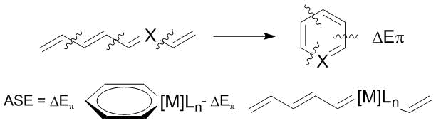
Scheme 3. Calculation of the aromatic stabilization energy (ASE) within the EDA approach.

The ASE-EDA approach which represents the development of the DRE computational method provides the numerical energetic evaluation of the conjugation and hyperconjugation effects in cyclic and acyclic systems [63]. The main advantage of this approach is the estimation of the π-effect along with the other EDA data such as the dissociation energy. The ASE-EDA values obtained by this method for benzene and pyridine are 42.5 and 45.7 kcal/mol, respectively [61], which differ from the classical ASE values of 34.1 and 31.0 kcal/mol, respectively [64]. The ASE-EDA method successfully demonstrated the aromaticity of metallabenzenes [61]. A drawback of this method, as well as the conventional ASE calculation scheme, is the necessity of constructing a reference system. Although the ASE-EDA method is not popular, it is of paramount importance for shaping the aromaticity concept.

In 2002 P. v. R. Schleyer suggested a versatile scheme for the energetic assessment of the π-aromaticity which allowed for overcoming some drawbacks. The calculation procedure [64] is very simple since it implies the estimation of a difference in the energies between a methyl derivative of the system under consideration and its obviously non-aromatic methylene isomer (Scheme 4). This isomerization scheme can be calculated at the very high theoretical levels (CCSD(T) or MP4(SDQ)), and the resulting value is called the isomerization stabilization energy (ISE) [64]. The ISE value can be calculated for any ring bearing at least one С=С double bond.

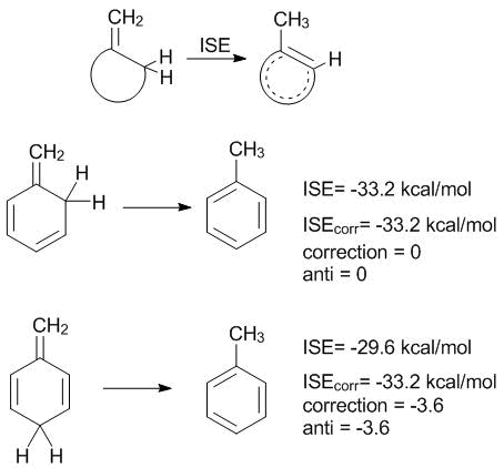
Scheme 4. Reactions used for evaluating the isomerization stabilization energy (ISE).

A peculiarity of the ISE criterion is that the calculation, for example, of benzene can be accomplished by two different methods that afford different energies (Scheme 4). The correction for syn- or anti-arrangement of CH₂ groups (–3.6 kcal/mol) must be introduced. In the case of naphthalene and pyridine, five and six isomerization reactions can be suggested, respectively [64]. After the introduction of corrections, the ISE_corr value almost does not depend on the isomer type used for calculations and amounts to one of the reliable energetic criteria. The ISE scheme became popular and works well for strained systems; the ISE values are in good agreement with other aromaticity criteria [35, 38, 64, 65].

Quite recently, a new scheme for the ASE assessment through the calculation of the energy of a homodesmic ring-opening reaction has been suggested (Scheme 5) [66]. This approach is applicable for both hydrocarbons and organic heterocycles, as well as metallabenzenes since a valence state of the heteroatom X does not change. An and Zhu [66] indicated the reliability of such an estimate of the ASE and its close value to the ISE data for low strain rings.

Scheme 5

At the current stage, all the energetic criteria are calculated only by quantum chemical methods; therefore, there are two parallel trends of the evolution of these criteria. The improvement of computational accuracy owing to the improvement of the theory level became possible after a giant leap in the productivity of computing machines. That is why the new values of the RE, ASE, and other parameters calculated by the high-level correlated methods have good reliability. In general, all the suggested energetic criteria require adaptation to a particular molecule, while in the case of metal clusters the energetic criteria are not applicable due to the impossibility even to present the reference molecules. Many schemes do not take into account the ring strain, hybridization changes, whereas the balanced ISE scheme describes only the π-effect. Therefore, the creation of new and advancing of the existing computational schemes for aromatic stabilization are required for the investigation of complex polyheterocyclic systems, as well as sigma- and three-dimensionally conjugated molecules interesting to modern science.

2.2. Structural criteria

In the development of the structural criteria, the original idea was that an aromatic ring consists of the bonds which are equalized or tend to equalize. In the case of benzene, this provides D_6h symmetry (although there is a dissenting opinion [67]), whereas the antiaromatic molecules retain bond alternation [34]. Therefore, it is believed that the higher the bond length equalization, the higher the degree of ring aromaticity.

There are several structural indices [34, 40], two of which are of current use. The index called the bond alternating coefficient (BAC) [68] is based on the calculation of a sum of the squares of the length differences (R_n) for sequential bonds:

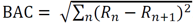(12)

where R_i is the length of the i bond in the ring under consideration. The closer the HOMA value to 1, the higher the aromaticity degree. If the molecule contains heteroatoms, then the bond lengths that involve them are defined through the Pauling bond order n_opt [71].The most popular and well-studied structural index is the harmonic oscillator model of aromaticity (HOMA) [9, 69], which is the evolution of the first structural Julg index A_J [70]. The HOMA index differs in the fact that the reference bond length R_opt is that of the energetically optimal bond, for which the shortening to a double bond and the elongation to a single one requires minimal energy:

(13)

(14)

The resulting bond order is recalculated to the equivalent bond length by the following formula:

r(N) = 1.467 – 0.1702 ln (nopt)

(15)

which is plugged into the HOMA formula (13). To accelerate and simplify the calculations, the known parameters for the most popular types of bonds are used (Table 2).

Table 2. HOMA structural parameters for the π-systems with heteroatoms [35]

Bond	R(1)	R(2)	Ropt	α	c	nopt
C–C	1.467	1.349	1.388	257.7	0.1702	1.590
C–N	1.645	1.269	1.334	93.52	0.2828	1.589
C–O	1.367	1.217	1.265	157.38	0.2164	1.602
C–P	1.814	1.640	1.698	118.91	0.2510	1.587
C–S	1.807	1.611	1.677	94.09	0.2828	1.584
N–N	1.420	1.254	1.309	130.33	0.2395	1.590
N–O	1.415	1.164	1.248	57.21	0.3621	1.586

nopt is the Pauling bond order for Ropt [70]

There is another modification of the HOMA method that involves the elongation (EN) and bond alternation (GEO) components. The calculations are performed according to the following formula [40]:

(16)

where R_av is the average interatomic distance in the ring.

The HOMA approach appeared to the highly successful not only for hydrocarbons, including polycyclic ones, but also for heterocycles. It afforded a good correlation with the energetic and magnetic criteria [34, 40]. One of the interesting features of the structural methods lies in the answer to the question: is there any molecule with higher structural aromaticity than that of benzene? The answer is that there is no such molecule [72], although the magnetic aromaticity (i.e., its assessment based on the magnetic criteria) can be even stronger. Of note is the report by Ostrowski and Dobrowolski [73], which is devoted to what the HOMA value shows. It was established that the HOMA index is not a simple aromaticity index. It also demonstrates the cyclic nature, the unsaturation degree, and the connection route of rings in polycyclic molecules. The HOMA ideology was widely used in the development of the electronic criteria (vide infra).

Obviously, the structural indices are empirical and mainly used for π-conjugated hydrocarbons and simple heterocyclic systems. There are a great variety of examples for which the described indices contradict other aromaticity criteria. Chen et al. reviewed this in 2005 [42]. The bond equalization was detected in strongly conjugated acyclic compounds. In contrast, the bond alternation in polyacenes was shown to be stronger than in the linear conjugated polyenes. Therefore, the structural factors do not always unambiguously indicate the manifestation of aromaticity. For complex heterocyclic, metallacyclic, and other systems, the structural criterion, i.e., the elongation of multiple bonds and the shortening of single bonds in a ring, can be anyway considered on a qualitative level. Within a series of structurally related molecules, quantitative analysis is possible.

2.3. Electronic criteria

Obedience to the electron counting rules 4n + 2 (Hückel) for planar molecules or 4n (Möbius) for twisted molecules is a fundamental criterion of aromaticity. These rules are stipulated by the configuration of molecular orbitals (MOs) and are necessarily fulfilled for aromatic rings. For other types of aromaticity, the electron counting rules may differ (Table 1). The indices based on the MO energy, such as the HRE, DRE, and REPE, refer to the energetic criteria (vide supra). The electronic criteria of aromaticity include the methods based on the investigation of electron localization/delocalization, which are usually divided into three groups [38]. The first one includes the conventional methods that deal with localized orbitals (BLW [57] and NBO [74] methods). The researchers should avoid the investigation of delocalized orbitals by the methods exploiting localized orbitals. The latter include all the valence bond methods, widely used methods such as NBO, NPA, and NLMO [74], as well as the methods in which the separation of orbitals by fragments can be ambiguous, for example, the local energy decomposition (LED) analysis [62]. Noteworthy, M. E. Volpin warned of the danger of application of the valence bond method for the investigation of aromaticity back in the 1960s [75].

One of the recent criteria, namely, the electron density of delocalized bonds (EDDB) [76] utilizes the advanced NBO approach:

(17)

where χ_μ(r) and χ_ν(r) are the wave functions, D^DB is the density matrix in the NBO basis. In this method, the decomposition of total electron density occurs by localized bond orbitals (two-center bonds and lone pairs) and delocalized bonds which represent a combination of three-center bonds. The latter are absent in the classical NBO theory. Ideologically the consideration of multicenter bonds is close to the earlier developed method of adaptive natural density partitioning (AdNDP) [77]. However, in the EDDB method, the decomposition by orbitals is automated and almost unambiguous. The AdNDP approach requires the manual introduction of multicenter and two-center bonds as well as the minimization of residual electron density.

According to Szczepanik, Solà, and coauthors [76, 78], the EDDB method has the following advantages: 1) the EDDB value does depend on a ring size; 2) the absence of parametrization and a necessity to construct model systems; 3) the EDDB analysis does not require high time expenditures; 4) this method is simple in application and interpretation since its shows the number of electrons which are effectively delocalized in a system. For quantitative analysis, the degree of delocalization is calculated as the ratio of the integral EDDB to the formal number of delocalized electrons (for benzene the delocalization degree is equal to 5.59/6 = 93%).

The realized script of the EDDB analysis (RunEDDB) allows one to calculate both the whole molecule and any fragment. There is also a possibility to take into account or not to take into account the local substituent effects, in particular, it is not recommended to involve hydrogen atoms in calculations [78]. Comparing all the EDDB results, it is necessary to substantiate the choice of a particular moiety, the consideration of certain orbitals and lone pairs.

An advantage of the EDDB method, as well as the methods that analyze the magnetic currents (CDA, vide infra), is the possibility of visualization of a conjugation route. For example, Fig. 2 shows the EDDB(r) isosurfaces for benzene and naphthalene, which present the usual forms of a π‑cloud. An indispensable part of the EDDB method is the analysis of natural orbitals of delocalized bonds (NODB), namely, their visualization and estimation of the population degree. Figure 3 depicts the NODB orbitals for benzene; the highest population of 1.78 e is characteristic of 3 π-orbitals. These NODB orbitals have certain similarities with canonical molecular orbitals (CMO), whereas the NBO orbitals do not resemble the CMОs.

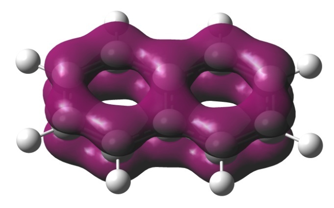
Figure 2. EDDB isosurfaces for benzene and naphthalene at a standard isovalue of 0.015 e.

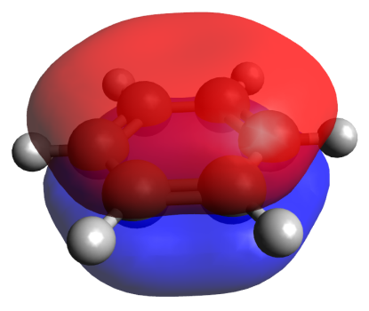
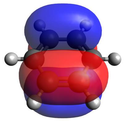
Figure 3. Natural orbitals of delocalized bonds (NODB) of π-type for benzene.

The EDDB criterion for a series of metallabenzenes [79], in which a conjugation chain completes the metal d-orbital and can afford the Hückel (4n+2) or Craig–Möbius (4n) aromaticity, allowed for defining the type of aromaticity. For planar metallacycles, the aromaticity rule was supplemented by the following statement [79]: if the HOMO level has the Möbius topology, then the realization of aromaticity requires the even number of π-type MOs, and if the HOMO exhibits the Hückel topology, the number of π-MOs must be odd. The EDDB method was tested for a series of standard systems; the correlations with the HOMA, FLU, and NICS(1) indices were established [78].

The modern electronic criteria include also the aromaticity indices of the second and third groups that are based on the distribution of electron density within Bader's quantum theory "Atoms in Molecules" (QTAIM) [80]. The primary QTAIM parameters such as the value of electron density ρ(r) and its Laplacian Dρ(r) at a bond critical point BCP (3;–1), the ellipticity index (EL) [81], as well as the values of ρ(r) and Dρ(r) at a ring critical point RCP (3;+1) [38] refer to the second group of methods. In some simple cases (i.e., for simple organic molecules), the correlation between these values and the popular HOMA, NICS, and ASE indices were observed [37, 38, 81]. Using the ideology of the structural index HOMA, based on ρ(r), the ellipticity (ε), and the bond length (R), the new index was suggested which was called the corrected total electron density (CTED) [82]:

(18) (19)

he value of is calculated by summing up the electron densities ρ_i at BCP, subtracting the corrected products of ellipticities ε_i and bond lengths R_i with ρ_i by all n bonds of the cyclic system. To calculate the CTED index itself, the value of is normalized according to equation 19, where the coefficient ζ is equal to 0.310947 based on the fact that the CTED value becomes zero for an ideal benzene molecule. This new index CTED can be attributed to the hybrid structural-electronic criteria; it demonstrated good reliability for polycyclic HCs [37–39, 82].

The application of the values of ρ(r) and Dρ(r) for the rings which involve heavy atoms is difficult since these QTAIM parameters strongly depend on the size of an electron shell and bond polarity. To eliminate such an undesired peculiarity, the delocalization indices (δ(A,B) or DIs) were suggested that refer to the third group of the methods [80]:

(20)

 where the integration of the density ρ_XC is performed over the atomic basins Ω_A and Ω_B.

The delocalization index for a pair of atoms δ(A,B) shows how many electron pairs are shared between the chosen atoms, and for a covalent bond, it is considered its order. The delocalization index is a theoretically well-founded characteristic of a chemical bond, without any assumption. The values of δ(A,B) are considered as alternatives to the bond lengths since they are not directly affected by the atomic radius. On the other hand, the DIs are the analogs of Mayer's bond order (MBO [83]); however, δ(A,B) is always less than the formal bond order 1, 2, or 3, and the greater a difference in the electronegativities of the bound atoms, the lower its value [84], which affords certain complications during interpretation.

The indices δ(A,B) were included in many approaches which utilize the bond lengths. For example, R. F. W. Bader introduced them into the HOMA index [85]. However, the fluctuation index (FLU) gained wider popularity [86]. The FLU index is based on the values of localization and delocalization indices: 

(21)

where δ(A_i) = S_{Aj ≠ Ai} δ(A_i,A_j)   and δ = 1  for A_i> A_j and δ =  –1 for A_i ≤ A_j . The FLU values are calculated using the parameters of С–С bonds (δ_ref) in benzene. Therefore, the FLU index provides a comparison of the aromaticity in the molecule under consideration relative to benzene. The lower the value of this index, the higher the aromaticity degree (for benzene FLU = 0). The modified index FLU_π was formulated soon after the introduction of this index, which takes into account only the π-delocalization.

Besides the index for simple two-center bonds δ(A,B) between adjacent atoms, the so-called para-index of delocalization (PDI) was suggested for six-membered rings, i.e., the calculation of δ(A,B) for carbon atoms located at the para-positions of a six-membered ring [87]. The PDI values reflect the delocalization in a six-membered ring. The higher the aromaticity degree, the higher its value (for benzene, PDI composes 0.105). To confirm this, good agreement between the PDI and other aromaticity criteria was demonstrated for hydrocarbons [37, 38, 86–88]. To improve the PDI index, Sablon et al. [89] suggested using the PDI values averaged over all atom pairs, which was called the pair-linear response (PLR). Mosquera et al. [90] proposed the application of multicenter delocalization indices (MDI) that can be calculated for all atoms in a ring. Although the MDI values are in good agreement with other topological parameters, they are almost not used as the aromaticity criteria due to complex and time-consuming calculations. Comparing the multicenter delocalization indices, it is important to remember their normalization [80].

Along with a variety of the delocalization indices based on the QTAIM theory, the approaches were developed that utilize the bond order indices MBO [83], the Mayer multicenter indices (MCI) [91], as well as I_ring index [92]. These indices also refer to the third group of the electronic criteria. For hydrocarbons, including polycyclic ones, good agreement between them is observed [38]. To compare the cycles differing in sizes, Giambiagi et al. suggested the method of MCI and I_ring normalization, which can be considered as separate indices [92]:                                    

(22) (23)

where N_π is the number of electrons in a ring, C is the constant equal to 1.5155, M is the ring size, and G(N_π) is the coefficient equal to 1 or –3 for aromatic and antiaromatic rings, respectively. The indices I_NB and I_NG worked well for a series of systems in the presence of heteroatoms, different ring sizes, system twist, etc. [38, 39, 92]. To calculate the values of I_NB and I_NG, the preliminary data on the aromatic or antiaromatic character is required in order to choose the correct coefficient G(N_π). The electronic indices MCI, I_ring, and their normalized analogs are hardly applicable for macrocycles. To eliminate this problem, the indices AV1245 and AV_min were suggested [93]. They represent the four-center MCI index for the atoms at positions 1, 2, 4, and 5 and its minimum among all the combinations of atoms in a ring, respectively. This approach offers an opportunity to estimate the delocalization degree in five-membered and larger rings without considerable time expenditures.

Earlier it was believed that the parameters in the QTAIM theory (electron density, its Laplacian, etc.) only slightly depend on the chosen theory level but this is not exactly true [94–96]. It is not surprising that the highest accuracy of topological parameters is demonstrated by the high-level correlated methods (MP4, CCSD(T), etc.), whereas, among the DFT functionals, the lowest errors are provided by PBE0 and SCAN. The most popular functional B3LYP can be not the best choice from the viewpoint of the QTAIM parameters [94]. To calculate the reliable δ(A,B) values, it is necessary to use the extended basis sets. For example, the widely used medium-size basis set Def2-TZVP can be insufficient [95]. It is worth recalling that the QTAIM parameters can be calculated based on the experimental electron density derived from the high-precision XRD data.

The computation of the QTAIM delocalization indices is a time-consuming process since it requires integration over a zero-flow surface. To accelerate the process, the application of an averaged shape of this surface was suggested, which was called the fuzzy atom approach [97]. This approach considerably accelerates the calculations (in 100 times and over) and does not lead to a significant loss in accuracy [98]. The delocalization indices calculated by this method were called fuzzy bond orders (FBO), which represent the simplified version of the delocalization indices. Both two- and multicenter FBOs are available.

The criteria based on the bond orders have received much attention in the last decade. Of note is the appearance of the new methods, AdNDP and EDDB, as well as the convenient instruments (MultiWFN [99] and ESI-3D [100] program packages) that allow for rapid and facile calculation of the bond order and delocalization indices.

The application of many electronic criteria is restricted: in some cases, the limitations are connected with parametrization, in other cases, the errors arise since the bond indices and DIs are strongly affected by different factors such as the bond polarity, steric effects, and ring strains. The changes in the DI or MBO are sometimes difficult to attribute to the manifestation of aromaticity. It is well known that the FLU and PDI values are distorted in the case of the presence of heteroatoms, whereas the MСI index does not work well for small rings [38]. However, one can offer the following versatile recommendation. First of all, to use the EDDB or AdNDP method. Secondly, due to the appearance of aromaticity, the bonds equalize and the δ(A,B) indices average as the bond orders, i.e., for double bonds the values of δ(A,B) reduce, while those for single bonds—increase. A case when the DI value is above 1 for a formally single bond in the conjugated ring can be considered as a preliminary confirmation of the existence of delocalization.

2.4. Magnetic criteria

To reveal the presence of aromaticity, of particular importance are the magnetic properties as most frequently used among others. M. Faraday discovered for the first time that benzene interacts with a magnetic field. This repulsion phenomenon was called diamagnetism. It laid the beginning of a description of aromaticity from the viewpoint of magnetic properties.

All the magnetic criteria can be divided into four groups that correspond to their development stages:

1. the experimental criteria (magnetic susceptibility, its anisotropy, and NMR chemical shifts) [41];

2. the calculated values of magnetic susceptibility exaltation and anisotropy, chemical shifts of ⁷Li and ³He nuclei [42];

3. the NICS (nucleus-independent chemical shift) method and its wide application [42];

4. the analysis of the density of magnetically induced currents (the CDA methods) [45, 46, 101].

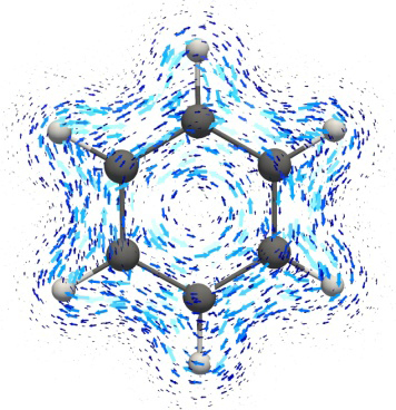
In 1910 Pascal [102] suggested the application of magnetic susceptibility constants to describe the relations between a molecule structure and the value of diamagnetic repulsion and indicated that this value for aromatic molecules is exalted, i.e., much higher than the one calculated by an additive scheme [44]. In 1936 Pauling explained the peculiar magnetic properties by the existence of induced ring currents of π-electrons (see Fig. 4) [103]. Later, London used the Hückel theory to calculate the magnetic susceptibility exaltation, which was called the London diamagnetism [104].

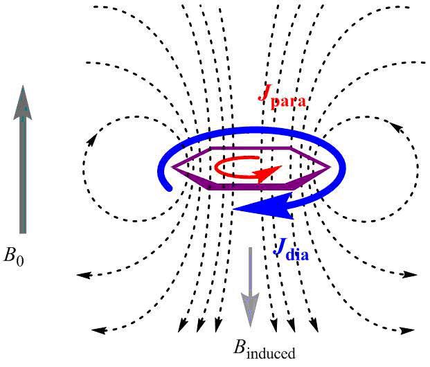
Figure 4. Scheme of magnetically induced currents that arise in a benzene ring upon application of an external magnetic field B₀: J_para are paratropic (moving clockwise) and J_dia are diatropic currents (moving counter-clockwise).

The availability of magnetic susceptibility constants facilitated the renewal of this criterion by Dauben et al. in the 1960s [105]. The diamagnetic susceptibility exaltation (Λ is a difference between the values of the experimental molar susceptibility (c_M) and that calculated by an additive scheme (c'_M ):

Λ = cM – c'M

(24)

If the compound exhibits significant magnetic susceptibility exaltation, it is aromatic (Table 3). Hence, this experimental criterion allows one to unambiguously judge the presence of aromaticity on a qualitative level. It was found that the value of Λ strongly depends on the ring size and the number of conjugating electrons [42]. In order to make a correct comparison between the values of Λ for different molecules, it is necessary to have an appropriate standard for calibration.

Table 3. Magnetic susceptibility exaltation (Λ 10^–6 cm³/mol) in conjugated hydrocarbons [106]

Compound	cM	cM′	Λ
Cyclohexene	57.5	8.3	–0.8
1,3-Cyclohexadiene	48.6	49.3	–0.7
Benzene	54.8	41.1	13.7
Naphthalene	91.9	61.4	30.5
Azulene	91.0	61.4	29.5
Chrysene	167	102	65
1,6-Methano[10]annulene	111.9	75.1	36.8
Pyrene	155	98	57
Trans-15,16-dimethyl-15,16-dihydropyrene	210	129	81

Flygare [106] detected significant anisotropy of magnetic susceptibility of aromatic molecules. The experimental measurement of this parameter was suggested as an aromaticity criterion. Several research groups tried to calculate the diamagnetic anisotropy since its measurement faces a series of experimental challenges. As a result, it was found that, for satisfactory coincidence with the experiment, a new term must be introduced that takes into account localized atomic contributions. Later it was shown that the same corrections are required for the calculation of magnetic susceptibility [42].

Another experimental criterion of aromaticity includes the chemical shifts in the NMR spectra [41, 42]. It was noted that the signals of the ring protons of aromatic compounds shift downfield relative to those of non-aromatic analogs. However, these shifts are not very large (~7.3 ppm for benzene, ~5.6 ppm for cyclohexene) [107]. At the same time, the chemical shifts of the protons located inside an annulene ring are strongly upfield shifted. Thus, the chemical shifts for the internal protons of [18]‑annulene compose –3.0 ppm, whereas those for the external protons are ~9.3 ppm; for the internal protons of a [18]‑annulene antiaromatic dianion, the chemical shifts are observed at 20.8 ppm and 29.5 ppm, while those for the external ones—at ca. –1.1 ppm [106]. At the modern level, the experimental magnetic criteria are almost not used (both the magnetic susceptibility exaltation and the chemical shifts) since the evaluation of magnetic properties of complex systems is difficult and there is no ambiguity in the choice of the reference values.

A transition from the experiment to calculations as a general tendency occurred also in the case of the magnetic criteria. In 1994 P. v. R. Schleyer suggested the magnetic criterion of aromaticity—the nucleus-independent chemical shift (NICS) [108]. Since then researchers stopped using the second group of criteria which include the calculated magnetic susceptibility exaltation and the chemical shifts of ⁷Li and ³He nuclei [41, 42].

From the mid-1990s, an era of the NICS indices (the third group of methods) began, which have not lost their popularity until now. The NICS represents the value (ppm) of absolute shielding at a space point. To calculate the NICS, the geometrical parameters of molecules are optimized, the hypothetical atoms Bq are placed at the points interesting for researchers, most frequently, in the ring center or above the ring center at some distances (usually 1 or 2 Å, Fig. 5), then, the values of absolute chemical shifts for the Bq atoms are calculated according to Schleyer's suggestion [108] using the GIAO method [104, 109] at the B3LYP/6-311+G* level of theory, and the resulting values are taken with opposite signs. The application of high-level correlated methods is possible (the perturbation and coupled-cluster theory) but the method recommended by P. v. R. Schleyer provides high reliability and is also rapid and convenient.

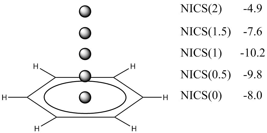
Figure 5. Arrangement of the Bq atoms during the calculation of the NICS indices for benzene.

The NICS criterion is formally very simple: the negative value evidences the aromaticity, while the positive one indicates the antiaromaticity of the molecule under consideration. Historically the first NICS(0) index was calculated by locating the Bq atom in the ring center. However, it was established that this index is not a pure characteristic of π-conjugation since it includes a contribution of the ring σ-bonds. In particular, this effect leads to a non-zero NICS(0) value even for obviously non-aromatic molecules, i.e., not all the rings that have the negative NICS indices are aromatic [110]. To exclude the σ-effect, the NICS(1) index was suggested, i.e., the NICS value at a distance of 1 Å above the ring center. Nevertheless, this  appeared to be insufficient. To improve the qualitative estimation of the aromaticity degree, the NICS methods underwent an evolutionary path [44] starting from single indices NICS(0) and NICS(1), and the application of zz-components to the construction of an isochemical shielding surface (ICSS). There is an additional separation of π- and σ-contributions, these values are called the dissected-NICS. Among them, the CMO-NICS method that utilizes the decomposition into π- and σ-components by the application of canonical molecular orbitals (CMOs) is quite physical; however, there is not always an opportunity to formally (and, hence, in an automated mode within the program code) to choose the orbitals by the π- and σ-types due to their mixed nature and/or the involvement of metal atom orbitals.

The advantages of the NICS method over other currently used aromaticity criteria consist in the simplicity of calculations, the absence of a necessity to introduce any corrections, to use references and calibration, as well as to have the preliminary data on the aromatic character [42]. The NICS method became the most popular aromaticity criterion. According to the Web of Science, nowadays, there are ~5000 reports that utilize the NICS concept. A good correlation between the NICS values, the geometrical parameters, and the magnetic susceptibility exaltation for a great number of compounds testify that the NICS indices are very efficient in the investigation of the aromaticity of organic molecules [42–44]. For aromatic hydrocarbons, a database of the NICS(0), NICS(1), NICS(0)_zz, and NICS(1)_zz values was created [111].

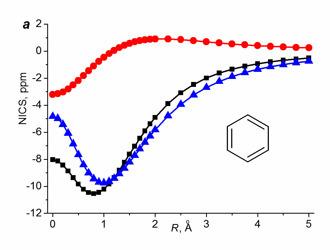
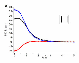
For non-benzenoid systems, it soon was established that the single NICS(0), NICS(1), and even NICS(1)_πzz values do not provide unambiguous assignment, in particular, for inorganic rings [112], metallacycles [61, 113], small rings [114], and polycyclic systems [44, 110], especially in the cases when the aromaticity degree is not high [112]. Despite this fact, the values of single NICS(0), NICS(1), and NICS(1)_zz are widely reported and compared. To solve the detected contradictions, several research groups suggested using two- [115–117] or three-dimensional [118] distribution of the NICS values in the vicinity of bonds of the ring under consideration. Among them, the most available approach is the NICS-scan method suggested by Stanger [115], which implies the construction of a dependence of the in-plane (NICS_in-plane = –⅓(σ_{xx +} σ_yy)) and out-of-plane (NICS_out-of-plane = NICS_zz = –⅓σ_zz) NICS components on the distance from the ring center. It must be mentioned that Stanger in his works [115–117] used the values of tensor components of magnetic shielding with reverse signs (–σ_ij) as the NICS indices, which is less convenient while comparing the NICS-scan curves with the single values NICS(0), NICS(1), or NICS(0)_zz. The NICS-scan method distinguishes well on a qualitative level the aromatic molecules from simply conjugated and antiaromatic ones. The criterion for π-aromatic rings is the presence of a minimum on the NICS_zz curve at distances differing from 0 Å (Fig. 6).

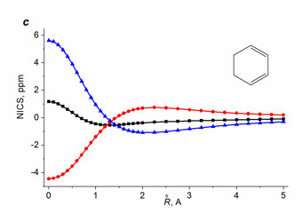Figure 6. NICS-scan curves for benzene (a), cyclobuta-1,3-diene (b), and cis-buta-1,3-diene; ■ – isotropic value,
●– in-plane (xx+yy) component, ▲– out-of-plane (zz) component.

Stanger also developed his own method for the application to polycyclic systems. The NICS-scan-XY method [117] was supplemented with scanning along the line that lies in a plane and cut across all the molecule rings. The interfering σ-contribution can be separated by the application of the CMO-NICS methods or sigma-model [116]. The sigma-model has essential drawbacks: first of all, in this method, a reference system deprived of the π-conjugation is played by the non-existing molecule. For benzene such a molecule is depicted in Fig. 7. It is not constructed naturally, instead, the hydrogen atoms are added to the unsaturated ring perpendicular to it at the conventional distance in order to make the ring saturated. Secondly, all the hydrogen atoms cannot be correctly added to the heteroatoms or metal atoms.

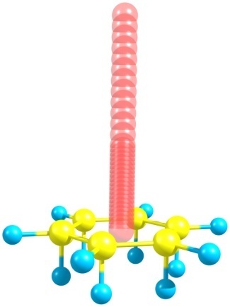
Figure 7. Reference model for benzene within the sigma-model approach [116]. Red circles refer to the Bq atoms.

The NICS-scan group of methods also includes the addition of Tiznado et al. [119], which implies the construction of a dependence of the NICS_zz component on the NICS_in-plane component. This dependence (NICS_in-out) very efficiently and clearly distinguishes the aromatic, non-aromatic, and antiaromatic rings (Fig. 8): for the aromatic rings, the curve lies strictly in the negative range of the NICS values. For a quantitative comparison, the NICS index free of the in-plane component (FiPC-NICS) was suggested that represents the NICS(R)_iso with the NICS_in-plane equal to zero.

Figure 8. NICS_in-out curves for typical aromatic, non-aromatic, and antiaromatic rings.

The ICSS method (NICS isosurface) and similar 2D NICS maps are quite popular methods [44] but they have limited opportunities and are essentially inferior in the amount of provided information than the CDA methods which should be preferred.

An alternative to all the NICS approaches can be considered the so-called aromatic ring current shielding (ARCS) method [120], which was suggested seven years earlier than the NICS-scan approach [115]. The ARCS method ideologically implies the calculation of the same magnetic shielding but in another way. The ARCS curve profile repeats the isotropic NICS-scan curve and exhibits similar features during the result interpretation. The ARCS method did not gain popularity since it appeared to be quite labor-consuming and poorly available; it is considered a predecessor to the CDA group of methods.

The fourth group of the magnetic criteria includes the CDA computational methods, according to which the distribution of induced currents (ICs) is analyzed as a reason for all the unusual magnetic properties of aromatic systems. These methods include anisotropy of the induced current density (ACID) [121], continuous transformation of the origin of the current density (CTOCD) [122], magnetically induced current density (MICD) [123], and gauge-including magnetically induced currents (GIMIC) [45, 124]. Historically the first method CTOCD [122], which appeared even before the NICS, describes the magnetic shielding insufficiently accurately; the errors can be reduced using the extended atomic basis sets, which has not been done earlier [125]. Despite the advanced theory (the recommended modification is CTOCD-DZ2) and availability within the SYSMOIC [126] and AIMAll [127] program packages, the CTOCD method is not used frequently [128–133]. The main achievement of the CTOCD approach is the visualization of ring currents and their demonstration in σ-aromatic cyclopropane [133]. In recent years, the SYSMOIC program is used to attempt the topological analysis of the IC density. In particular, the application of a stagnation graph [129] was suggested that shows the lines and critical points where the IC density is close to zero.

Another popular CDA method consists in the calculation of the anisotropy of a magnetic shielding tensor, which was called the anisotropy of the induced current density (ACID, sometimes AICD) [121]:

(25)

where J_jⁱ(r)  are the components of the magnetic shielding tensor.

From the phenomenological point of view, it was assumed that, in the case of conjugated and aromatic systems, the shielding anisotropy essentially increases in the vicinity of conjugated bonds. Geuenich et al. [121] reviewed the successful application of the ACID method for conventional systems. Figure 9 shows the ACID isosurfaces for benzene, thiophene, and naphthalene, which clearly reflect the conjugation routes invariant relative to the vector B₀. It should be noted that the ACID approach does not differentiate aromatic and antiaromatic rings; therefore, the analysis of ring current directions is required. Until 2014 (before the release of the Gaussian09 D.01 program), the ACID method had a formidable technical problem of a compilation of the modified Gaussian program code; therefore, it was used very rarely. Despite the improvement of the ACID approach by the introduction of the precise GIAO theory, Nozawa et al. [134] showed on the examples of porphyrins that the ACID method provides an incorrect conjugation route; therefore, the ACID data should be checked carefully and correlate with the results of other criteria.

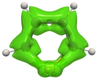
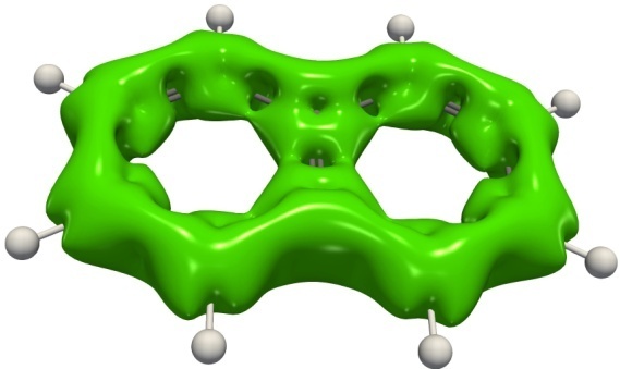
Figure 9. Isosurfaces of the ACID function for benzene, thiophene, and naphthalene.

The development of the CTOCD method by the introduction of the GIAO theory [104] led to the formation of the MICD approach [123]. However, slightly earlier (2004) Sundholm suggested the GIMIC method [45, 101, 124] that has a stricter and more developed theory than the other CDA methods:

(26)

The GIMIC equation for the calculation of IC ( ) utilizes a single-electron density matrix D _μν  and a magnetically excited density matrix in an atomic basis. These matrices are calculated during the conventional computation of the magnetic shielding constants. The derivatives and estimate the electronic interaction of an external magnetic field with a nucleus; ϵ_ντβ is the three-dimensional Levi–Civita symbol that excludes the repetition.

In general, the CTOCD, MICD, and GIMIC methods, despite the differences in theory and realization, provide the same information [101]. The only advantage of the ACID and CTOCD methods is the possibility of separating the contributions by CMO, which realization within the GIMIC method is only in the planning stage.

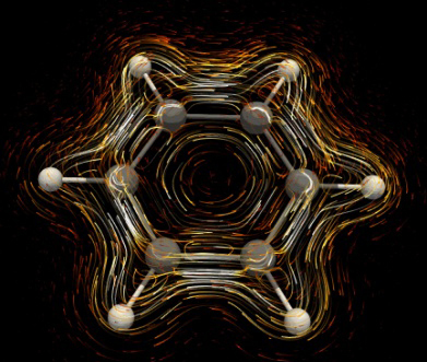
The visualization of ring currents and thereby an aromatic conjugation route can be performed by several means [45]: using the isosurfaces separately for dia- (blue) and paramagnetic (red) contributions (Fig. 10), the most popular method—using a vector map (Fig. 11а) [122, 123, 135]), and using a map of vectors joined by isolines (IC streamlines, Fig. 11b). For aromatic rings, the diamagnetic (aromatic) ICs are located outside the ring (blue in Fig. 10). Their isosurface (usually presented as a result of the GIMIC method) has a closed contour and prevails over the paramagnetic current isosurface (red), which is inside the ring. The discovery of the CDA methods was that the ring diamagnetic currents lie not only under and above the ring, repeating a shape of the π-cloud, but also beyond it and in its plane, which is most clearly demonstrated in Ref. [124]. In the case of the presence of only hydrogen substituents in the ring, the isosurface of diamagnetic ICs is likely to bend round the C–H bonds.

Figure 10. Isosurface of the IC module for the diatropic (blue) and paratropic (red) contributions for a benzene molecule.

a	b

Figure 11. Methods for visualization of magnetically induced currents in the form of vector maps (a)
and IC streamlines (b) by the example of a benzene molecule.

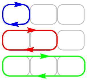
It is well known that simple single bonds also possess magnetic properties which are caused by the appearance of magnetic currents of the bonds and atoms. They can be distinguished from the ring aromatic currents using the IC streamline maps (Fig. 11), this most modern method for visualization can be accomplished in an animated version, its application is required for complex systems. The advantages of the analysis of IC streamlines were clearly highlighted [101, 135–137]. Furthermore, the IC streamlines allow one to reveal the local, semilocal, and global ring currents (Fig. 12) in the case of polycyclic systems [101].

	Local current
	Semilocal current
	Global current

Figure 12. Illustration of the application of local, semilocal, and global ring currents for polycyclic systems.

In order to estimate quantitatively and thereby to compare the aromaticity degrees of different rings, the integration of the IC density is used. The integration plane is chosen perpendicular to the ring plane and the bond under consideration and passing through the center of this bond (Fig. 13). Table 4 lists the values of ring current strength for some conventional molecules. Due to the closed character of the ring current, the value of IRCS in a monocyclic molecule principally does not depend on the bond choice but some errors are possible in practice. The errors in the IRCS estimates can be caused by the choice of the integration plane as well as the involvement of atoms and bonds of adjacent substituents. Therefore, the bulky substituents in the ring under investigation should be replaced for methyl groups or better for H, which is also more convenient during the visual analysis of the IC distribution.

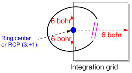
Figure 13. Scheme of integration of magnetically induced currents.

The GIMIC method, as well as the NICS approach, can be applied to any molecular system at any level of theory; reliable results are available at the DFT level, in particular, the B3LYP/Def2-TZVP method was recommended [138]. The GIMIC method was used to demonstrate the aromaticity of a wide range of polyheterocycles [139, 141], inorganic clusters [142], some metallacycles [143, 144], twisted annulenes [145], and nanoobjects [146, 147]. The interesting fact is that an aromatic route in fullerene С₆₀ does not encompass all the bonds in rings [148], which is caused by the compensation of ring currents of fused rings. In antiaromatic cyclophane, three-dimensional aromaticity was shown [135]. The correlations between the data of the GIMIC, NICS, and other methods were observed. However, having gained sufficient data, it was established that the current strength (IRCS) depends on the ring size [45].

Table 4. IRCS values for conventional organic molecules calculated at the B3LYP/Def2-TZVP level [136, 138–141]

Molecule	IRCS, nA/T
Cyclopropene	6.7
Cyclopropane	10.0
Cyclobutadiene	–19.9
Cyclopentadiene	5.4
Cyclopentadienyl anion	12.9
Benzene	11.8
Cyclohexane	0.2
Cycloheptatriene	6.1
Tropylium cation	12.9
Naphthalene	12.9
Pyridine	11.6
Pyrrole	11.6
Furan	10.3
Thiophene	11.6

The disadvantage of all the CDA methods is the complicated interpretation of their results and their dependence on the direction of B₀. For example, upon consideration of the IC distribution on a qualitative level, it is not always possible to unambiguously distinguish the π- and σ-aromaticity. The calculation of the IC integral values can be accompanied by distortions owing to the local ICs of multiatomic substituents and sometimes even that of a methyl group. Furthermore, the values of current strength (IRCS) depend on the ring size. In the case of the CTOCD method, additional errors may appear due to the imperfect character of the underlying theory. To simplify the interpretation of the IC density, the application of the IC vorticity tensor, its trace [149], or anisotropy [150] was suggested. Along with this, the approaches to the topological analysis of the IC density were formulated, in particular, analysis of critical points and stagnation graphs. These are quite new approaches that require thorough checking on a broad series of conventional molecules.

2.5. Optical spectroscopy criteria

Optical spectroscopy (UV-vis, IR, and Raman) as the aromaticity criteria comprises the group of rare experimental criteria and utilizes several parameters.

The first group of parameters includes the wavelength (l_max) and the intensity of absorption bands which are registered in the electronic absorption spectra in the UV and visible regions. The value of l_max is analogous to the comparison of the energetic values HMG (vide supra); therefore, the application of l_max of the band as well as its intensity in the investigations on aromaticity is correct only provided several conditions. It is possible to compare the transitions of the same nature (for example, p–p* transitions) between the molecular orbitals of close structures and thereby for structurally related molecules. For aromatic compounds, an increase in l_max and the intensity of these transitions must be observed owing to an increase in the polarization capacity [47]. The successful application of these parameters was reported in several works for simple hydrocarbons and heterocycles [151–158].

The second group includes the parameters of vibrational spectroscopy. On the one hand, these are the experimental vibration frequencies and their intensities in the Raman spectra [49], on the other hand—the force constants [48].

Studying p-aromaticity, Cremer et al. [48] introduced the force constants recalculated to the bond orders into the HOMA concept. For this purpose, the following four stages should be proceeded: 1) the recalculation of vibration frequencies into force constants in order to get free of the frequency dependences on the atom masses; 2) the calculation of local (pair) force constants n_i by the kinematic decomposition of normal coordinates, which reflect the internal strength of a particular chemical bond; 3) the recalculation of local force constants into relative bond orders via the introduction of an appropriate reference model (n_opt); 4) the calculation of the AI_vib index by plugging the resulting bond orders into formula (27) analogous to the HOMA equation (13):

(27)

The ring is considered aromatic if the AI_vib value ranges within 0.5 and the AI_vib rate for benzene equal to 0.924. For a broad series of polycyclic hydrocarbons, it was shown that the AI_vib criterion qualitatively confirms the anti-, non-, or aromatic character of rings but there are quantitative divergences between the AI_vib and HOMA index [48].

Guo et al. [159] and Han et al. [160] used the frequency of a breathing ring mode as an aromaticity criterion: the higher the frequency, the higher the aromaticity degree. This criterion is quite unreliable since the vibration frequency mainly depends on its shape, which is affected by the presence of substituents and heteroatoms, atom masses, ring sizes, and aromaticity last.

The application of the Raman line intensities is based on the fact that the Raman spectra are sensitive to the presence of conjugation [49, 161, 162]. As it was demonstrated in the classical works of P. P. Shorygin [49, 162–164], the presence of conjugation in a molecule leads to a reduction in the frequency (owing to a reduction in the bond order) and a significant increase in the intensity of polarized Raman lines which correspond to the symmetrical stretching vibrations of conjugated multiple bonds. For example, Shorygin [164] revealed that the intensity of the Raman lines that corresponds to the stretching vibration of butadiene double bonds is almost ten times higher than that of alkenes, and a further increase in the number of conjugated double bonds leads to progressive intensity growth [164].

The intensities of the Raman lines are determined by the components of a derivative of the polarization capacity α by the normal vibrational coordinate Q_i (δα_σ/δQ_i)₀. In the semiclassical approximation of P. P. Shorygin, the value of the polarizability derivative components is defined by the following equation:

(28)

where ν_e is the frequency of the electron transition 0 → e, ν is the frequency of the laser exciting radiation line, and (M_σ)_0e is a matrix element of the dipole moment of the electron transition 0 → e. The conjugation in a molecule leads to a reduction in the value of ν_e of the most low-lying electron transition (compared to that for a non-conjugated analog) and, hence, to approaching of ν_e and ν. At the presence of a difference between the frequencies ν_e and ν below 50000 cm^–1 (the so-called pre-resonance conditions), the intensity of the polarized lines in the Raman spectrum, which refer to the symmetrical vibrations of the bonds involved in the conjugation, start to increase [49, 164]. The closer the values of ν and ν_e, the greater this increase. It was found that the main role in equation (28) is played by the second term and, hence, a prerequisite for the realization of pre-resonance conditions is a non-zero value of the derivative δν_e/δQ_i, which is connected with a change in the molecular geometry in the excited state.

2.6. Availability of the computational criteria of aromaticity

The electronic, structural, and energetic criteria are based on the main molecular parameters (geometry, energy, CMO parameters, and electron density distribution); therefore, they can be calculated at any available level of theory using a wide range of programs. The most versatile programs are as follows: ORCA [165], Gamess US [166], CFOUR [167], MRCC [168], Priroda [169], Gamess Firefly [170], OpenMolCAS [171], Dalton/LSDalton [172], and NWChem [173]. They are free and generally accessible, whereas the programs such as Gaussian [174], Turbomole [175], ADF [176], MOLPRO [177], and QChem [178] are commercial. All the programs for calculation of electronic criteria have versatile formats for data insertion (for example, Molden, WFN, and WFX), the scripts and programs for further calculations (for example, AIMAll [127], MultiWFN [99], and Molden2AIM [179]). For the energetic parameters, it is very important to use the high-level theories such as QCISD, CCSD, MP4(SDQ), or even higher since the accuracy of the rapid and available DFT method may be insufficient, especially in the case of the appearance of high-spin states [180]. All the quantum chemists try to use only the DFT methods since the high-level correlated methods require huge computational capacity and time expenditures; furthermore, they have considerable software limitations. It also should be noted that among the diversity of DFT functionals, in recent years, the range-separated functionals were recommended for the description of delocalization effects [181].

The main structural and electronic criteria such as the Bird, Julg (A_j), HOMA, AdNDP, CTED, PDI, FBO, MCI, and FLU indices are available in the MutliWFN program which was initially specialized for the QTAIM analysis. I_ring and the MCI indices are available in the ESI‑3D program [99]. Hence, both of these programs provide almost all the requirements in the electronic and structural criteria. The EDDB criterion in recent times has received public availability within the RunEDDB script [182]. Although this program uses the input data which can be provided by many quantum-chemical programs, the realization of RunEDDB is made so that the application of the EDDB criterion is possible only using the calculations in the Gaussian program.

The EDA method for calculation of the versatile EDA-ASE energetic criterion is implemented only in the expensive and poorly available program ADF. An alternative to the original EDA method can be the following closely related methods: the natural orbitals for chemical valence (NOCV) [183] and local energy decomposition (LED) [184]. They are available in the free program ORCA; however, the NOCV and LED methods are not used for the investigation of aromaticity.

The NICS indices gained the highest popularity owing to the simplicity of calculations, the availability of the commercial Gaussian program and the B3LYP functional. In turn, the CMO-NICS or LMO-NICS calculations are rather labor-consuming and are available only within the commercial NBO code starting from version 5 [185]. The NBO program (the current version is 7) is inexpensive and quite popular; therefore, the results of the CMO-NICS analysis as well as the separation of their values into diamagnetic and paramagnetic contributions are published regularly. The authors of the NICS-scan and sigma-model NICS suggest the script [186] that allows for automated calculations by the NICS-scan method in combination with the CMO-NICS approach in the Gaussian and NBO6 programs.

The CDA methods require the greatest computational experience since they require several sequential steps (geometry optimization, calculation of magnetic shielding constants, calculation of induced currents) which are completed by different methods for visualization of the results. These methods are gaining popularity. The GIMIC method has the interfaces to the Gaussian, TurboMole, QChem, CFOUR, ACES, Fermion++, and Dalton/LSDalton programs, which in total allow for computing the IC density at any level of theory. On the other hand, the computational procedure by the GIMIC method is simple for adoption, it has high-quality documentation, and the output data of the GIMIC method are provided in the open formats which can be clearly and qualitatively visualized by all the known methods in cross-platforms of the generally available programs ParaView [187], GNUPlot [188], VMD [189], and JMOL [190]. The competitive method MICD is available only in the highly specialized but generally accessible program Dirac [191]. The calculation by the CTOCD method and visualization of the corresponding results can be carried out with the SYSMOIC package [126]; a standard WFX file of electron density is used, which can be obtained with the Gaussian program or others.

In general, there are two main trends. On the one hand, the calculations become progressively more complicated. On the other hand, new multifunctional, open, generally accessible and free codes are created that provide automation and thereby simplify the computational process for researchers.

3. Aromaticity in organoelement and organometallic compounds

Recently, the investigations on the aromaticity effect have turned to the field of organoelement and organometallic chemistry. Thus, the planar boron-containing clusters [134, 192–195], metal clusters [196, 197], metallabenzenes [61, 77, 113], metallaheterobenzenes [198–200], and other metallacycles of transition metals [201–203], in particular, metallapentalenes [143, 144, 204–208] which display the Hückel or Craig–Möbius aromaticity were reported. Recently, the chemistry and electronic structures of non-planar and spyro-metallacycles have been reviewed by Zhang et al. [209]. A series of bimetallic complexes with two amidinate ligands, in which a multiple М–М bond was assumed, was studied by a variety of computational methods [210, 211]. The results obtained showed that the Hückel aromaticity degree increases on replacing the metal atom moving down a group. Continuous attention is drawn to aromaticity in the excited state [23, 192, 212–214]. Aromaticity of the formally strained metallacycles of the fourth group [25, 215, 216] and a series of mono- [26, 217] and bicyclic tetrylenes [217–224] was studied. Hence, the following two main directions can be outlined in the investigations on aromaticity: (1) elucidation of aromaticity and estimation of its degree in new compounds, (2) evaluation of the aromaticity degree in the earlier known compounds using new methods. In most cases, a set of the used criteria is limited to 2–3 from the traditional ones: the ASE, ISE, NICS, HOMA, ACID, or PDI indices. Advanced methods such as the GIMIC, MICD, EDDB, and AdNDP approaches are only gaining popularity. It should be noted that the existence of reliable criteria has already afforded new types of aromaticity such as the adaptive [23] and mс-M–C aromaticity [24, 25] which are caused exclusively by the involvement of metal atoms in a conjugation. Furthermore, it was demonstrated that metallacyclobutadienes, unlike organic analogs, are stabilized owing to the aromaticity effect [225–227].

At the current stage of development of the aromaticity criteria, the most urgent methods for investigations are the following ones: the ASE, ISE, HOMA, BAC, and all possible modifications of the NICS, CTOCD, MICD, GIMIC, ACID, AdNDP, EDDB, MCI, PDI, and I_ring. The number of reports devoted to establishing the peculiarities of modern methods and their applicability is not so high. Many authors, presenting the developed criterion, compared the results with the most popular methods at that moment. Thus, the following methods were presented: the FLU [86], PDI [87], EDDB [76, 78], FiPC-NICS [119], HOMA [34, 35], ISE [64], I_ring [92], MCI [91], AV1245 [93], and GIMIC [101, 124] indices. Most of the reports explore the correlations of the NICS indices with the structural, electronic, and energetic criteria. On a rather large series of organic molecules and metal clusters, it was shown that the HOMA and FLU criteria should not be used for analyzing aromaticity during chemical reactions [214, 228]. The NICS indices should be excluded from a comparison of the rings of different dimensions and sizes, bearing different atoms. Although Feixas et al. [214] believe that the electronic criteria (FLU, MCI, PDI, etc.) provide the highest reliability, they should be carefully applied in the case of non-planar distortions of rings and the presence of heteroatoms differing in nature. It is underscored that the calculations by the MCI method require high theory levels (MP4, CCSD). In the case of inorganic rings, the aromaticity evaluation must be thoroughly analyzed. Among the diversity of the NICS indices for the evaluation of π-aromaticity, the most reliable method according to the Feixas et al. [214] is the NICS(0)_πzz method. Since the NICS and MCI indices do not include any reference parameters they are applicable for the investigation of metal-containing molecules, including metal clusters. These molecules can exhibit double aromaticity; therefore, it is recommended to use the separation by π- and σ-contributions of the MCI and NICS as well as to apply the Stanger NICS-scan method [228]. In a well-cited report [229], while comparing C₆H₆, C₄N₂H₆, and N₆H₆²⁺ (i.e., a very narrow set), it was concluded that the ring current strength IRCS is not applicable for the evaluation of aromaticity. This conclusion causes doubts since during the analysis of the IRCS correlation with the energetic criterion, the energy of aromatic stabilization was estimated by the most non-standard and biased method.

The existence of a possibility to compare different molecules determines the applicability of one or another criterion. Thus, for complex heterocyclic molecules and, in particular, organometallic compounds, the non-parametrized criteria can be used; among them, the most popular ones are the ASE, ISE, NICS, ACID, EDDB, CTOCD, AdNDP, and GIMIC indices. In our opinion, the preferred methods are the EDDB instead of the AdNDP and the GIMIC instead of the CTOCD owing to the more advanced theory.

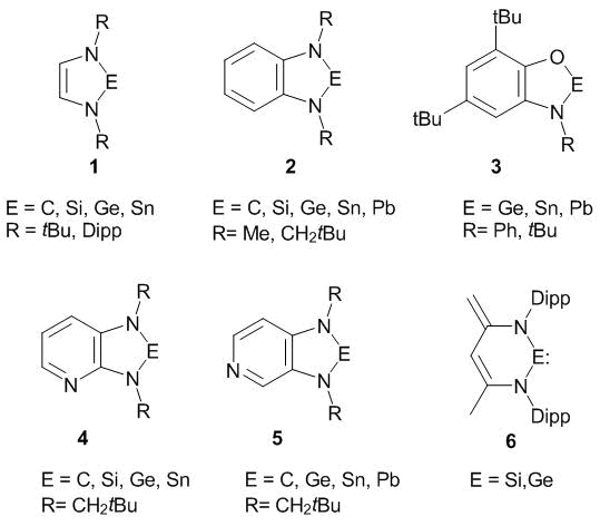
A complex of the criteria that includes the ISE, ACID, GIMIC, EDDB, and NICS-scan indices and the parameters of the UV-vis and Raman spectra was tested for a series of N-heterocyclic tetrylenes 1–6 (Scheme 6) [217–224]. Silylene and germylene of type 6 appeared to be non-aromatic despite the fact that they can be presented in a zwitterion form with six π-electrons [220]. The number of π-electrons in 1–5 corresponds to the Hückel rule 4n + 2, which causes π-type aromaticity in them. This was confirmed by all the methods except for the ACID. It was found that the value of the ACID function for heavier tetrylenes 1–5E (E = Si, Ge, Sn, and Pb) in the vicinity of the E–N bonds is very low and is comparable to those for usual σ-bonds [219]. Formally, the ACID criterion refutes the existence of aromaticity in five-membered rings of 1–5E (E = Si, Ge, Sn, and Pb) which involve the metal atom. This contradicts all the rest data. Therefore, taking into account the results of works [134, 221], the ACID method is not recommended for the application. The conclusions about aromaticity based only on the ACID method, for example, in Refs. [143, 144, 230] should be considered insufficiently reliable.

Scheme 6

While studying delocalization in 1–4, the undesirable peculiarity of the EDDB method was detected [223, 224]. Upon visualization of the EDDB(r) function in the region of the heavy atom E = Si, Ge, Sn, or Pb at the conventional isovalue of 0.015 ē, the isosurface interrupts (lilac in Fig. 14), at the lower isovalue of 0.005 ē, it closes (cyan). This peculiarity of the EDDB(r) function does not affect the quantitative parameters EDDB_H or EDDB_F and the shapes of the NODB orbitals. Of note is also the insufficient accuracy of the EDDB method for estimation of the σ-conjugation [207].

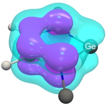
Figure 14. Isosurface of the EDDB(r) function at two isovalues: 0.015 ē (lilac) and 0.005 ē (cyan) for germylene 1Ge.

Upon application of the experimental criteria of vibrational spectroscopy (the frequency of С=С vibrations and the intensity of the corresponding line in the Raman spectra), it was shown that their use is possible owing to the presence of appropriate vibrations in 1–5, which do not involve the atom E what is extremely important [217, 219, 222, 224]. Furthermore, for 1–5 the UV-vis criterion (the wavelength of π–π* transition) could also be applied. The optical spectroscopy criteria demonstrated a general tendency of an increase in the aromaticity degree in 1–5 on passing from Е = C to Pb. It should be noted that the spectral criteria displayed higher sensitivity compared to other computational methods. The results of the calculation criteria ISE, EDDB, NICS-scan, and GIMIC for 1–5 revealed both coincidences and contradictions. Since the physical properties that underlie the methods are different, the effects of additional factors also differ. The sequences based on the electronic criterion EDDB and the energetic criterion ISE for tetrylenes 2–5 coincide and indicate the tendency of the increasing π-aromaticity degree from С to Pb, which coincides with the data of the optical spectra. The tendency of aromaticity strengthening on moving down the group is caused by an increase in the Lewis acidity [224] and polarizability of the E atom in the same order. All the criteria show that in the series of heavier tetrylenes 1–5, there is observed a gradual increase in the aromaticity degree from Si to Pb, when carbenes 1С–5С can adopt both the beginning and end of the series. The series C > Si ~ Ge ~ Sn ~ Pb based on the magnetic criteria NICS and GIMIC does not coincide with the series based on the other methods. As it was already mentioned, the ring current value (IRCS) depends on the ring size: the larger the ring, the weaker the current. Therefore, the five-membered ring in carbenes 1C–5C, under other conditions being equal, must possess a higher current strength than their heavier analogs. The effect of the ring size on the IRCS upon such a comparison appears to be greater than a change in the aromaticity, which explains the opposition of the magnetic series to the other ones, although it coincides with intuitive chemical expectations of the higher aromaticity degree of carbenes 1C–5C. At the same time, the ring size in 1–5 increases from Si to Ge, Sn, and Pb, and the IRCS values slightly increase in the same sequence. In this case, the weakening effect of the current strength from Si to Pb appears to be low; therefore, the values of the IRCS correspond to the general tendency of aromaticity strengthening while moving down the group.

It is obvious that the IRCS parameter can be used to compare the degree of aromaticity of the rings featuring similar sizes. The analysis of the IRCS data for tetrylenes 1–5 (Table 5) showed that for each element E = C, Si, Ge, Sn, and Pb a single aromaticity series is obtained: 1 > 2 ~ 5 ~ 4 > 3, i.e., the five-membered rings in 1 possess the highest aromaticity degree; benzannulated derivatives 2, pyrido-annulated compounds 4 and 5 only slightly differ from each other; and the aromaticity degree of amidophenolates 3 is the lowest one. An important peculiarity of bicyclic molecules 2–5 is the presence of a united 10-π-electronic aromaticity; therefore, the aromaticity weakening in the five-membered ring is compensated by the benzene/pyridine ring. The vibrational spectroscopy parameters do not allow one to make an analogous direct comparison due to differences in the shapes of vibrations of molecules 1–5. It should be noted that the positions of the absorption bands that correspond to the π–π* transition in monomeric derivatives 2, 3, and 4 are very close, which does not contradict the data of the GIMIC and EDDB methods.

Table 5. NICS-scan (ppm), IRCS (nA/T), λ(π–π*) (nm), and EDDB (e) values for tetrylenes 1–5 [217, 218, 221–223]

Molecule	NICzz minimum	FiPC-NICS	IRCS	π-EDDB	EDDBFa	λ(π–π*)b
1C	-8.1	-5.9	10.4	2.54	2.94	224
2C	–7.1	–5.9	8.2	6.91	2.10	248
4C	–7.5	–4.7	9.6	7.28	2.50	244
5C	–7.6	–5.2	9.7	7.00	2.47
1Si	–5.8	–5.6	8.7	2.33	2.73	312
2Si	–5.0	–4.9	6.8	6.98	2.31	326
4Si	–4.4	–4.2	7.0	7.25	2.35	324
5Si	–4.5	–4.4	7.1	7.16	2.28
1Ge	–6.0	–5.9	8.9	2.67	3.06	346
2Ge	-5.4	–5.7	7.9	7.17	2.52	360
3Ge	–5.0	–5.0	7.1	6.70	1.92	360
4Ge	–4.8	-4.7	7.6	7.49	2.54	360
5Ge	–4.9	–4.8	7.6	7.32	2.46
1Sn	–5.1	–5.05	8.6	2.87	3.23	454
2Sn	–5.1	–5.13	7.8	7.34	2.62	430
3Sn	–4.7	–4.7	7.0	6.80	2.05	448
4Sn	–4.4	–4.4	7.4	7.68	2.54	437
5Sn	–4.4	–4.4	7.4	7.42	2.48
2Pb	–4.8	–4.77	7.8	7.51	2.67	500
3Pb	–4.7	–4.6	7.1	6.92	2.19	530
4Pb	–4.3	–4.3	7.5	7.67	2.54
5Pb	–4.3	–4.3	7.5	7.53	2.54

а the EDDBF values are presented for the five-membered ring; b the experimental values.

A comparison of the data on the aromaticity of 1–5 [217–224] with their reactivity [231–236] shows that there are no foundations to fully correlate a pure effect of aromaticity with the reactivity. A similar conclusion was drawn a long time ago for organic polycyclic molecules [237]. The aromaticity effect in tetrylenes 1–5 according to the EDDB data corresponds to the delocalization degree ranging from ~30 to ~50%, which affords the additional energetic stabilization (the values of ISE range from ~10 to ~20 kcal/mol). In general, the aromaticity effect in 1–5 is much weaker than in the classical aromatic compounds (benzene, pyridine, and thiophene) and has a secondary effect on their reactivity. Carbenes by their chemical behavior always differ from the heavier analogs since the reactivity is affected to a larger extent by the strength of bonds, basicity (carbenes possess significantly higher basicity), chemical rigidity, redox potential, increase in the stability of divalent state from С to Pb, as well as the peculiarities of each Е^II element, for example, the propensity for disproportionation (characteristic of the Sn and Pb compounds). It should also be underscored that the aromaticity in tetrylenes 1–5 shields the vacant p_z-orbital of the E atom, which leads to its inability/weakened ability to coordinate the Lewis bases (THF, MeCN). Upon dissolution, non-aromatic dimers 2Sn (R = Me) [218] and 3Sn, 3Pb [223] dissociate, at the same time, aromaticity is recovered, which compensates the dimerization energy.

A complex of the ISE, GIMIC, delocalization indices, NICS-scan, and vibrational spectroscopy criteria passed through a complicated methodological verification during the investigation of metallacyclopropenes 7 and 8 (Scheme 7) [215]. It was shown that the elongation of the С=С bond with the simultaneous elongation of the Е/M–C bonds (structural criterion), a reduction in the C=C delocalization index with a simultaneous increase in the analogous values for the E/M–C bonds (electronic criterion), a reduction in the frequency of νC=C (optical criterion), and the negative values of the isomerization stabilization energy (energetic criterion), in general, are similar for both types of the molecules and can be considered as a consequence of the existence of aromaticity in them, which was assumed earlier [216, 238]. It should be noted that the vibrational spectroscopy criterion is strictly inapplicable to cyclopropenes 7 and 8 since the so-called νC=C vibration involves the Е or М atom, which causes, under other conditions being equal, a reduction in the frequency of this vibration and growth of the intensity of the corresponding Raman line [215]. The presence of aromaticity in 7 and 8 was determined by the analysis of magnetic currents within the GIMIC method. Thus, in 7 there is a diatropic magnetic current, which is absent in 8; therefore, rings 7 display aromaticity (σ-type at E = С and pseudo-π-type at Е = Si, Ge), whereas cyclopropenes 8 (М = Ti, Zr, Hf) are non-aromatic cyclic compounds. An explanation to this observation was based on the analysis of molecular orbitals; for 7 it was presented as early as 25 years ago [239] and is in good agreement with all observations. The orbital overlapping pattern in 8 was described earlier [216]; however, the authors did not take into account the fact that the additional π-overlapping in a three-membered ring is prohibited by symmetry; therefore, π-aromaticity in 8 assumed in [216] is absent.

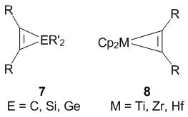
Scheme 7

Analyzing the NICS-scan and NICS_in-out data for three-membered organic and organoelement rings, a phenomenological dependence was detected that allows one to assume an aromaticity type with a high probability. Thus, the π-aromatic rings afford a minimum on the NICS_out-of-plane curve at R ≠ 0 Å (Fig. 6а) and the shape of an inverted arch of the NICS_in-out curve (Fig. 15а). In the case of σ-aromaticity, the NICS_in-out curve appears to be straightened on one side (Fig. 15b) [215]. In general, the evaluation of aromaticity in three-membered rings is quite a complicated task that requires careful consideration.

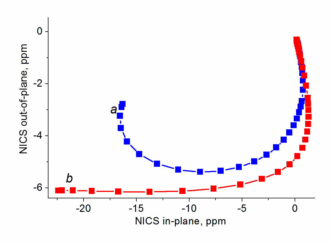
Figure 15. Shape of the NICS_in-out curve characteristic of π- (а) and σ-type (b) aromaticity
by the example of silacyclopropene and cyclopropene, respectively [222].

Within the NICS theory, the quantitative analysis of rings can be carried out using the FIPC-NICS value [119], which is valid for evaluation of π-aromaticity, or the minimum on the NICS_in-out curve for other types of aromaticity [25]. During the analysis of the NICS-scan curves for aromatic tetrylenes 1 and 2 [218, 219], it was noted that the distance from the ring center, which corresponds to the NICS_zz curve minimum, increases from 1.0 Å (E = C) to 1.3 Å (E = Sn) as the E atom size grows. Therefore, for organic rings, the NICS_zz minimum corresponds to the conventional NICS(1)_zz index, while for the metal-containing rings, a comparison of the min-NICS_zz values more accurately and better corresponds to the IRCS data [218, 219, 221].

The ISE and NICS-scan criteria were used simultaneously with the GIMIC and EDDB methods to study the aromatic properties of molecules 9–11 (Scheme 8) [25, 26, 240]. A new type of mc-M–C-aromaticity was discovered in these compounds, which is realized owing to the conjugation of multicenter metal–carbon bonds. The changes in the aromaticity degree upon substitution of the E atom for 9 and 10 demonstrate the same tendency as was observed for tetrylenes 1–5, i.e., its strengthening on moving down the group. In the case of pyramidanes 9 (E = Ge, Sn, Pb), this tendency coincides with a reduction in the frequencies and growth of the Raman line intensities that correspond to the С₄-base vibrations [241]. The CMO and NODB analysis revealed that the mc-M–C-aromaticity obeys the conventional rules 4n + 2 for 9 and 11, which is analogous to the results of the report of Schleyer [14]. It should be underscored that the ISE and NICS criteria appeared to be inefficient for the investigation of delocalization of the fourth group metallacycles [25, 215].

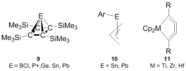
Scheme 8

The presence of a metal atom in the conjugation system can lead to the appearance of not only the Hückel aromaticity [61] but also the Craig–Möbius [113], f-orbital [13], adaptive [23], or triple aromaticity [15]. The new mс-М–С delocalization type in allyltetrylenes 10 is caused by the conjugation of four electrons in a four-membered ring [25], which in some extent resembles the four-electron aromaticity in planar B₄-clusters [192, 242], whereas the four-electron aromaticity in metallacyclobutadienes has π-character [225, 226].

The approaches based on the NICS, EDDB, and GIMIC methods applied to metallapentalenes 12–14 (Scheme 9) [243, 244] allowed for revealing that the strong donor ligands at the electron-deficient metal center facilitate the appearance of adaptive π-aromaticity. In the case of Re and Os pentalenes, significant tolerance to the donor ligands was demonstrated. In the presence of electron-withdrawing ligands, aromaticity in the excited state of Os pentalenes and pentalynes arises more rarely [243]. The addition of a three-membered ring to pentalenes, i.e., a cyclopropene moiety in 15, a selenirene ring in 16, and a methylenecyclopropene moiety in 17 causes the appearance of σ-aromaticity [144, 244–246].

Scheme 9. Aromatic metallapentalenes and their derivatives.

4. Conclusions

The effect of aromaticity, the cyclic delocalization of electrons, can be obscured/distorted by other electronic effects, while the metal atom, due to wider possibilities of orbital overlapping, facilitates the appearance of non-conventional aromaticity. Therefore, it is necessary to use as many criteria as possible [4] and not to forget to consider the experimental criteria and reactivity. The magnetic criteria have certain features in a quantitative comparison, which restricts the elucidation of different molecules. However, the resulting diamagnetic current, especially strong, arises just due to the aromaticity effect. To define the type of aromaticity, we recommend analyzing the topology of a resulting diamagnetic ring current, which can be carried out more conveniently and reliably within the GIMIC method. The location of the diamagnetic current at some distance from the ring plane (~1 Å) is indicative of π-delocalization, whereas the arrangement in the ring plane evidences σ-aromaticity. A special type of mc-M–C-aromaticity in a plane is characterized by the presence of a diamagnetic current both outside and inside the ring. In the case of three-dimensional delocalization, the IC distribution at all the non-equivalent directions of the external magnetic field should be considered. The conclusions about the type of aromaticity based on the analysis of magnetic currents must be confirmed by the results of the analysis of delocalized NODB orbitals and their population. The analysis of this type of orbitals compared to the analysis of canonical molecular orbitals has an advantage that consists in simple interpretation. The number of highly populated NODB orbitals indicates the number of electrons that take part in delocalization, their shape indicates the type (p-, σ-, or other) of cyclic conjugation. A sum of the NODB population degrees is a quantitative characteristic of the delocalization degree.

The development of aromaticity criteria and the accumulation of knowledge about it leads to the fact that, nowadays, many authors call into question the idea about the multidimensional nature of aromaticity but underscore the diversity of its manifestation. This is reflected in the fact that there are continuous attempts to arrange a single series by the aromaticity degree, first of all, for the classical p-aromatic compounds, and to reveal direct correlations and to explain the collisions between the data of different criteria.

Acknowledgements

This work was supported by the Ministry of Science and Higher Education of the Russian Federation.

Electronic supplementary information

Electronic supplementary information (ESI) available online: the visualization procedure of the NICS, EDDB, ACID, and GIMIC results. For ESI, see DOI: 10.32931/io2125r

References

1. Aromaticity. Modern Computational Methods and Applications, I. Fernandez (Ed.), 2021, Elsevier, Amsterdam. DOI: 10.1016/C2019-0-04193-3
2. IUPAC. Compendium of Chemical Terminology, 2nd ed. (the "Gold Book"), A. D. McNaught, A. Wilkinson (Eds.), Blackwell Sci. Publ., Oxford, 1997. DOI: 10.1351/goldbook.A00442
3. P. v. R. Schleyer, Chem. Rev., 2001, 101, 1115–1118. DOI: 10.1021/cr0103221
4. P. v. R. Schleyer, Chem. Rev., 2005, 105, 3433–3435. DOI: 10.1021/cr030095y
5. N. Martín, L. T. Scott, Chem. Soc. Rev., 2015, 44, 6397–6400. DOI: 10.1039/C5CS90085A
6. (a) E. Hückel, Z. Physik, 1931, 70, 104–186; (b) E. Hückel, Z. Physik, 1931, 72, 310–337; (c) E. Hückel, Z. Physik, 1932, 76, 628–648.
7. E. Heilbronner, Tetrahedron Lett., 1964, 5, 1923–1928. DOI: 10.1016/S0040-4039(01)89474-0
8. R. Breslow, Chem. Eng. News, 1965, 43, 90–100.
9. M. G. Evans, E. Warhurst, Trans. Faraday Soc., 1938, 34, 614–624. DOI: 10.1039/TF9383400614
10. (a) M. J. S. Dewar, Bull. Soc. Chim. Belg., 1979, 88, 957–967. DOI: 10.1002/bscb.19790881201; (b) M. J. S. Dewar, M. L. McKee, Pure Appl. Chem., 1980, 52, 1431–1441. DOI: 10.1351/pac198052061431; (c) M. J. S. Dewar, J. Am. Chem. Soc., 1984, 106, 669–682. DOI: 10.1021/ja00315a036
11. D. P. Craig, N. L. Paddock, Nature, 1958, 181, 1052–1053. DOI: 10.1038/1811052a0
12. C. S. Wannere, C. Corninboeuf, Z.-X. Wang, M. D. Wodrich, R. B. King, P. v. R. Schleyer, J. Am. Chem. Soc., 2005, 127, 5701–5705. DOI: 10.1021/ja042716q
13. A. C. Tsipis, C. E. Kefalidis, C. A. Tsipis., J. Am. Chem. Soc., 2008, 130, 9144–9155. DOI: 10.1021/ja802344z
14. J. Chandrasekhar, E. D. Jemmis, P. v. R. Schleyer, Tetrahedron Lett., 1979, 20, 3707–3710. DOI: 10.1016/S0040-4039(01)95503-0
15. B. B. Averkiev, A. I. Boldyrev, J. Phys. Chem. A, 2007, 111, 12864–12866. DOI: 10.1021/jp077528b
16. A. B. McEwen, P. v. R. Schleyer, J. Org. Chem., 1986, 51, 4357–4368. DOI: 10.1021/jo00373a006
17. J. Aihara, J. Am. Chem. Soc., 1978, 100, 3339–3342. DOI: 10.1021/ja00479a015
18. K. Wade, J. Chem. Soc. D, 1971, 792–793. DOI: 10.1039/C29710000792
19. D. M. P. Mingos, Nature, Phys. Sci., 1972, 236, 99–102. DOI: 10.1038/physci236099a0
20. S. Winstein, J. Am. Chem. Soc., 1959, 81, 6524–6525. DOI: 10.1021/ja01533a052
21. D. J. Sagl, J. C. Martin, J. Am. Chem. Soc., 1988, 110, 5827–5833. DOI: 10.1021/ja00225a038
22. H.-J. Zhai, B. B. Averkiev, D. Yu. Zubarev, L.-S. Wang, A. I. Boldyrev, Angew. Chem., Int. Ed., 2007, 46, 4277–4280. DOI: 10.1002/anie.200700442
23. D. Chen, T. Shen, K. An, J. Zhu, Commun. Chem., 2018, 1, 18. DOI: 10.1038/s42004-018-0018-y
24. N. C. Baird, J. Am. Chem. Soc., 1972, 94, 4941–4948. DOI: 10.1021/ja00769a025
25. R. R. Aysin, S. S. Bukalov, J. Mol. Struct., 2021, 1242, 130735. DOI: 10.1016/j.molstruc.2021.130735
26. R. R. Aysin, S. S. Bukalov, Organometallics, 2021, 40, 938–497. DOI: 10.1021/acs.organomet.1c00050
27. D. L. Thorn, R. Hoffmann, Nouv. J. Chim., 1979, 3, 39–45.
28. E. D. Jemmis, P. v. R. Schleyer, J. Am. Chem. Soc., 1982, 104, 4781–4788. DOI: 10.1021/ja00382a008
29. A. Hirsch, Z. Chen, H. Jiao, Angew. Chem., Int. Ed., 2000, 39, 3915–3917. DOI: 10.1002/1521-3773(20001103)39:21<3915::AID-ANIE3915>3.0.CO;2-O
30. J. Poater, M. Solà, Chem. Commun., 2011, 47, 11647–11649. DOI: 10.1039/C1CC14958J
31. T. B. Tai, R. W. A. Havenith, J. L. Teunissen, A. R. Dok, S. D. Hallaert, M. T. Nguyen, A. Ceulemans, Inorg. Chem., 2013, 52, 10595–10600. DOI: 10.1021/ic401596s
32. H. T. Pham, L. V. Duong, M. T. Nguyen, J. Phys. Chem. C, 2014, 118, 24181–24187. DOI: 10.1021/jp507901n
33. P. Cui, H.-S. Hu, B. Zhao, J. T. Miller, P. Cheng, J. Li, Nat. Commun., 2015, 6, 6331. DOI: 10.1038/ncomms7331
34. T. M. Krygowski, M. K. Cyrański, Chem. Rev., 2001, 101, 1385–1420. DOI: 10.1021/cr990326u
35. M. K. Cyrański, Chem. Rev., 2005, 105, 3773–3811. DOI: 10.1021/cr0300845
36. M. Alonso, I. Fernández, in: Aromaticity. Modern Computational Methods and Applications, I. Fernandez (Ed.), 2021, Elsevier, Amsterdam, ch. 6, pp. 195–235. DOI: 10.1016/B978-0-12-822723-7.00006-6
37. M. Poater, M. Duran, M. Solà, B. Silvi, Chem. Rev., 2005, 105, 3911–3947. DOI: 10.1021/cr030085x
38. F. Feixas, E. Matito, J. Poater, M. Solà, Chem. Soc. Rev., 2015, 44, 6434–6451. DOI: 10.1039/c5cs00066a
39. I. Casademont-Reig, E. Ramos-Cordoba, M. Torrent-Sucarrat, E. Matito, in: Aromaticity. Modern Computational Methods and Applications, I. Fernandez (Ed.), 2021, Elsevier, Amsterdam, ch. 7, pp. 235–259. DOI: 10.1016/B978-0-12-822723-7.00007-8
40. H. Szatylowicz, P. A. Wieczorkiewicz, T. M. Krygowski, in: Aromaticity. Modern Computational Methods and Applications, I. Fernandez (Ed.), 2021, Elsevier, Amsterdam, ch. 3, pp. 71–99. DOI: 10.1016/B978-0-12-822723-7.00003-0
41. R. H. Mitchell, Chem. Rev., 2001, 101, 1301–1316. DOI: 10.1021/cr990359
42. Z. Chen, C. S. Wannere, C. Corminboeuf, R. Puchta, P. v. R. Schleyer, Chem. Rev., 2005, 105, 3842–3888. DOI: 10.1021/cr030088
43. R. Gershoni-Poranne, A. Stanger, Chem. Soc. Rev., 2015, 44, 6597–6615. DOI: 10.1039/c5cs00114e
44. R. Gershoni-Poranne, A. Stanger, in: Aromaticity. Modern Computational Methods and Applications, I. Fernandez (Ed.), 2021, Elsevier, Amsterdam, ch. 4, pp. 99–154. DOI: 10.1016/B978-0-12-822723-7.00004-2
45. M. Dimitrova, D. Sundholm, in: Aromaticity. Modern Computational Methods and Applications, I. Fernandez (Ed.), 2021, Elsevier, Amsterdam, ch. 5, pp. 155–194. DOI: 10.1016/B978-0-12-822723-7.00005-4
46. D. Geuenich, K. Hess, F. Köhler, R. Herges, Chem. Rev., 2005, 105, 3758–3772. DOI: 10.1021/cr0300901
47. M. V. Vol'kenshtein, Structure and Physical Properties of Molecules, Izd. AN SSSR, Moscow, 1955, pp. 463–465 [in Russian].
48. D. Setiawan, E. Kraka, D. Cremer, J. Org. Chem., 2016, 81, 9669–9686. DOI: 10.1021/acs.joc.6b01761
49. P. P. Shorygin, K. Ya. Burshtein, Russ. Chem. Rev., 1991, 60, 1–24. DOI: 10.1070/RC1991v060n01ABEH001028
50. S. W. Slayden, J. F. Liebman, Chem. Rev., 2001, 101, 1541–1566. DOI: 10.1021/cr990324
51. M. K. Cyrański, P. v. R. Schleyer, T. M. Krygowski, H. Jiao, G. Hohlneicher, Tetrahedron, 2003, 59, 1657–1665. DOI: 10.1016/S0040-4020(03)00137-6
52. P. v. R. Schleyer, M. Manoharan, H. Jiao, F. Stahl, Org. Lett., 2001, 3, 3643–3646. DOI: 10.1021/ol016553b
53. C. H. Suresh, N. Koga, J. Org. Chem., 2002, 67, 1965–1968. DOI: 10.1021/jo010903q
54. M. K. Cyrañski, T. M. Krygowski, A. R. Katritzky, P. v. R. Schleyer, J. Org. Chem., 2002, 67, 1333–1338. DOI: 10.1021/jo016255s
55. L. J. Schaad, B. A. Hess, Chem. Rev., 2001, 101, 1465–1476. DOI: 10.1021/cr9903609
56. F. De Proft, P. Geerlings, Chem. Rev., 2001, 101, 1451–1464. DOI: 10.1021/cr9903205
57. R. C. Haddon, T. Fukunaga, Tetrahedron Lett., 1980, 21, 1191–1192. DOI: 10.1016/S0040-4039(00)71367-0
58. A. Minsky, A. Y. Meyer, M. Rabinovitz, Tetrahedron, 1985, 41, 785–791. DOI: 10.1016/S0040-4020(01)96458-0
59. C. W. Bird, Tetrahedron, 1985, 41, 1409–1414. DOI: 10.1016/S0040-4020(01)96543-3
60. P. Fowler, Nature, 1991, 350, 20–21. DOI: 10.1038/350020a0
61. I. Fernández, G. Frenking, G. Merino, Chem. Soc. Rev., 2015, 44, 6452–6463. DOI: 10.1039/c5cs00004a
62. A. Kovács, C. Esterhuysen, G. Frenking, Chem. Eur. J., 2005, 11, 1813–1825. DOI: 10.1002/chem.200400525
63. D. Cappel, S. Tüllmann, A. Krapp, G. Frenking, Angew. Chem., Int. Ed., 2005, 44, 3617–3620. DOI: 10.1002/anie.200500452
64. P. v. R. Schleyer, F. Pühlhofer, Org. Lett., 2002, 4, 2873–2876. DOI: 10.1021/ol0261332
65. A. Tokatlı, F. Ucun, J. Phys. Org. Chem., 2014, 27, 380–386. DOI: 10.1002/poc.3274
66. K. An, J. Zhu, J. Organomet. Chem., 2018, 864, 81–87. DOI: 10.1016/j.jorganchem.2018.01.038
67. S. Shaik, A. Shurki, D. Danovich, P. C. Hiberty, Chem. Rev., 2001, 101, 1501–1540. DOI: 10.1021/cr990363l
68. T. M. Krygowski, A. Ciesielski, M. Cyrański, Chem. Pap., 1995, 49, 128–132.
69. J. Kruszewski, T. M. Krygowski, Tetrahedron Lett., 1972, 13, 3839–3842. DOI: 10.1016/S0040-4039(01)94175-9
70. A. Julg, P. François, Theor. Chim. Acta, 1967, 8, 249–259. DOI: 10.1007/BF00527311
71. L. Pauling, J. Am. Chem. Soc., 1947, 69, 542–553. DOI: 10.1021/ja01195a024
72. J. Cz. Dobrowolski, ACS Omega, 2019, 4, 18699–18710. DOI: 10.1021/acsomega.9b02628
73. S. Ostrowski, J. Cz. Dobrowolski, RSC Adv., 2014, 4, 44158–44161. DOI: 10.1039/c4ra06652a
74. E. D. Glendening, C. R. Landis, F. Weinhold, WIREs Comput. Mol. Sci., 2012, 2, 1–42. DOI: 10.1002/wcms.51
75. M. E. Volpin, Yu. D. Koreshkov, V. G. Dulova, D. N. Kursanov, Tetrahedron, 1962, 18, 107–122. DOI: 10.1016/0040-4020(62)80030-1
76. D. W. Szczepanik, M. Solà, in: Aromaticity. Modern Computational Methods and Applications, I. Fernandez (Ed.), 2021, Elsevier, Amsterdam, ch. 8, pp. 259–284. DOI: 10.1016/B978-0-12-822723-7.00008-X
77. D. Yu. Zubarev, A. I. Boldyrev, Phys. Chem. Chem. Phys., 2008, 10, 5207–5217. DOI: 10.1039/B804083D
78. D. W. Szczepanik, M. Andrzejak, J. Dominikowska, B. Pawełek, T. M. Krygowski, H. Szatylowicz, M. Solà, Phys. Chem. Chem. Phys., 2017, 19, 28970–28981. DOI: 10.1039/c7cp06114e
79. D. W. Szczepanik, M. Solà, ChemistryOpen, 2019, 8, 219–227. DOI: 10.1002/open.201900014
80. R. F. W. Bader, Atoms in Molecules. A Quantum Theory, Clarendon Press, Oxford, 1990.
81. J. Dominikowska, M. Palusiak, Struct. Chem., 2012, 23, 1173–1183. DOI: 10.1007/s11224-011-9941-6
82. A. Tokatlı, F. Ucun, J. Phys. Org. Chem., 2014, 27, 380–386. DOI: 10.1002/poc.3274
83. I. Mayer, Chem. Phys. Lett., 1983, 97, 270–274. DOI: 10.1016/0009-2614(83)80005-0
84. D. B. Chesnut, Chem. Phys., 2001, 27, 9–16. DOI: 10.1016/S0301-0104(01)00425-6
85. X. Fradera, M. A. Austen, R. F. W. Bader, J. Phys. Chem. A, 1999, 103, 304–314. DOI: 10.1021/jp983362q
86. E. Matito, M. Duran, M. Sola, J. Chem. Phys., 2005, 122, 014109. DOI: 10.1063/1.1824895
87. J. Poater, X. Fradera, M. Duran, M. Solà, Chem. Eur. J., 2003, 9, 400–406. DOI: 10.1002/chem.200390041
88. P. Bultinck, Faraday Discuss., 2007, 135, 347–365. DOI: 10.1039/B609640A
89. N. Sablon, F. De Proft, M. Solà, P. Geerlings, Phys. Chem. Chem. Phys., 2012, 14, 3960–3967. DOI: 10.1039/C2CP23372J
90. M. Mandado, P. Bultinck, M. J. González-Moa, R. A. Mosquera, Chem. Phys. Lett., 2006, 433, 5–9. DOI: 10.1016/j.cplett.2006.11.009
91. R. Ponec, I. Mayer, J. Phys. Chem. A, 1997, 101, 1738–1741. DOI: 10.1021/jp962510e
92. M. Giambiagi, M. S. de Giambiagi, C. D. dos Santos Silva, A. P. de Figueiredo, Phys. Chem. Chem. Phys., 2000, 2, 3381–3392. DOI: 10.1039/B002009P
93. E. Matito, Phys. Chem. Chem. Phys., 2016, 18, 11839–11846. DOI: 10.1039/c6cp00636a
94. M. G. Medvedev, I. S. Bushmarinov, J. Sun, J. P. Perdew, K. A. Lyssenko, Science, 2017, 355, 49–52. DOI: 10.1126/science.aah5975
95. Y.-G. Wang, C. Matta, N. H. Werstiuk, J. Comput. Chem., 2003, 24, 1720–1729. DOI: 10.1002/jcc.10435
96. M. Jabłonski, M. Palusiak, J. Phys. Chem. A, 2010, 114, 2240–2244. DOI: 10.1021/jp911047s
97. I. Mayer, P. Salvador, Chem. Phys. Lett., 2004, 383, 368–375. DOI: 10.1016/j.cplett.2003.11.048
98. E. Matito, J. Poater, M. Solà, M. Duran, P. Salvador, J. Phys. Chem. A, 2005, 109, 9904–9910. DOI: 10.1021/jp0538464
99. Multiwfn program, http://sobereva.com/multiwfn/
100. E. Matito, Electron Sharing Indexes Program for 3D Molecular Space Partition (ESI-3D), http://iqcc.udg.edu/~eduard/ESI/
101. D. Sundholm, H. Fliegl, R. J. F. Berger, WIREs Comput. Mol. Sci., 2016, 6, 639–678. DOI: 10.1002/wcms.1270
102. G. A. Bain, J. F. Berry, J. Chem. Educ., 2008, 85, 532–536. DOI: 10.1021/ed085p532
103. L. Pauling, J. Chem. Phys., 1936, 4, 673–677. DOI: 10.1063/1.1749766
104. F. London, J. Phys. Radium, 1937, 8, 397–409. DOI: 10.1051/jphysrad:01937008010039700
105. H. J. Dauben Jr., J. D. Wilson, J. L. Laity, J. Am. Chem. Soc., 1968, 90, 811–813. DOI: 10.1021/ja01005a059
106. W. H. Flygare, Chem. Rev., 1974, 74, 653–687. DOI: 10.1021/cr60292a003
107. F. Faglioni, A. Ligabue, S. Pelloni, A. Soncini, R. G. Viglione, M. B. Ferraro, R. Zanasi, P. Lazzeretti, Org. Lett., 2005, 7, 3457–3460. DOI: 10.1021/ol051103v
108. P. v. R. Schleyer, C. Maerker, A. Dransfeld, H. Jiao, N. J. R. van Eikema Hommes, J. Am. Chem. Soc., 1996, 118, 6317–6318. DOI: 10.1021/ja960582d
109. T. Helgaker, M. Jaszuński, K. Ruud, Chem. Rev., 1999, 99, 293–352. DOI: 10.1021/cr960017t
110. R. Islas, G. Martínez-Guajardo, J.O.C. Jiménez-Halla, M. Solà, G. Merino, J. Chem. Theory Comput., 2010, 6, 1131–1135. DOI: 10.1021/ct100098c
111. F. Alvarez-Ramírez, Y. Ruiz-Morales, J. Chem. Inf. Model., 2020, 60, 611–620. DOI: 10.1021/acs.jcim.9b00909
112. J. O. C. Jiménez-Halla, E. Matito, J. Robles, M. Solà, J. Organomet. Chem., 2006, 691, 4359–4366. DOI: 10.1016/j.jorganchem.2006.01.038
113. M. Mauksch, S. B. Tsogoeva, Chem. Eur. J., 2018, 24, 10059–10063. DOI: 10.1002/chem.201802270
114. J. Wu, X. Liu, Y. Hao, H. Chen, P. Su, W. Wu, J. Zhu, Chem. Asian J., 2018, 13, 3691–3696. DOI: 10.1002/asia.201801279
115. A. Stanger, J. Org. Chem., 2006, 71, 883–893. DOI: 10.1021/jo051746o
116. A. Stanger, J. Org. Chem., 2010, 75, 2281–2288. DOI: 10.1021/jo1000753
117. R. Gershoni-Poranne, A. Stanger, Chem. Eur. J., 2014, 20, 5673–5688. DOI: 10.1002/chem.201304307
118. T. Heine, C. Corminboeuf, G. Seifert, Chem. Rev., 2005, 105, 3889–3910. DOI: 10.1021/cr030082k
119. J. J. Torres-Vega, A. Vásquez-Espinal, J. Caballero, M. L. Valenzuela, L. Alvarez-Thon, E. Osorio, W. Tiznado, Inorg. Chem., 2014, 53, 3579–3585. DOI: 10.1021/ic4030684
120. J. Jusélius, D. Sundholm, Phys. Chem. Chem. Phys., 1999, 1, 3429–3435. DOI: 10.1039/A903847G
121. D. Geuenich, K. Hess, F. Köhler, R. Herges, Chem. Rev., 2005, 105, 3758–3772. DOI: 10.1021/cr0300901
122. S. Coriani, P. Lazzeretti, M. Malagoli, R. Zanasi, Theor. Chim. Acta, 1994, 89, 181–192. DOI: 10.1007/BF01132801
123. S. Pathak, R. Bast, K. Ruud, J. Chem. Theory Comput., 2013, 9, 2189–2198. DOI: 10.1021/ct3011198
124. J. Jusélius, D. Sundholm, J. Gauss, J. Chem. Phys., 2004, 121, 3952–3963. DOI: 10.1063/1.1773136
125. J. R. Cheeseman, G. W. Trucks, T. A. Keith, M. J. Frisch, J. Chem. Phys., 1996, 104, 5497–5509. DOI: 10.1063/1.471789
126. http://sysmoic.chem.unisa.it/MANUAL/S1.html
127. AIMAll (Version 19.10.12), T. A. Keith, TK Gristmill Software, Overland Park KS, USA, 2019 (http://aim.tkgristmill.com).
128. S. Pan, R. Saha, S. Mandal, P. K. Chattaraj, Phys. Chem. Chem. Phys., 2016, 18, 11661–11676. DOI: 10.1039/C5CP06282A
129. R. J. F. Berger , G. Monaco, R. Zanasi, J. Chem. Phys., 2020, 152, 194101. DOI: 10.1063/5.0006992
130. S. Pelloni, F. Faglioni, R. Zanasi, P. Lazzeretti, Phys. Rev. A, 2006, 74, 012506. DOI: 10.1103/PhysRevA.74.012506
131. S. Pelloni, P. Lazzeretti, Int. J. Quantum Chem., 2011, 111, 356–367. DOI: 10.1002/qua.22658
132. H. T. Pham, M. T. Nguyen, J. Phys. Chem. A, 2018, 122, 1378–1391. DOI: 10.1021/acs.jpca.7b11191
133. P.W. Fowler, J. Baker, M. Lillington, Theor. Chem. Acc., 2007, 118, 123–127. DOI: 10.1007/s00214-007-0253-2
134. 134      R. Nozawa, J. Kim, J. Oh, A. Lamping, Y. Wang, S. Shimizu, I. Hisaki, T. Kowalczyk, H. Fliegl, D. Kim, H. Shinokubo, Nat. Commun., 2019, 10, 3576. DOI: 10.1038/s41467-019-11467-4
135. H. Fliegl, J. Jusélius, D. Sundholm, J. Phys. Chem. A, 2016, 120, 5658–5664. DOI: 10.1021/acs.jpca.6b03950
136. R. R. Valiev, H. Fliegl, D. Sundholm, Phys. Chem. Chem. Phys., 2018, 20, 17705–17713. DOI: 10.1039/c8cp03112f
137. L. Alvarez-Thon, W. Caimanque-Aguilar, Chem. Phys. Lett., 2017, 671, 118–123. DOI: 10.1016/j.cplett.2017.01.027
138. H. Fliegl, S. Taubert, O. Lehtonen, D. Sundholm, Phys. Chem. Chem. Phys., 2011, 13, 20500–20518. DOI: 10.1039/C1CP21812C
139. H. Fliegl, R. Valiev, F. Pichierri, D. Sundholm, Chemical Modelling, M. Springborg, J.-O. Joswig (Eds.), 2018, vol. 14, pp. 1–42. DOI: 10.1039/9781788010719-00001
140. H. Fliegl, D. Sundholm,^, S. Taubert, J. Jusélius, W. Klopper, J. Phys. Chem. A, 2009, 113, 8668–8676. DOI: 10.1021/jp9029776
141. C. Kumar, H. Fliegl, D. Sundholm, J. Phys. Chem. A, 2017, 121, 7282–7289. DOI: 10.1021/acs.jpca.7b07607
142. Y.-C. Lin, J. Jusélius, D. Sundholm, J. Gauss, J. Chem. Phys., 2005, 122, 214308. DOI: 10.1063/1.1924590
143. C. Zhu, M. Luo, Q. Zhu, J. Zhu, P. v. R. Schleyer, J. I.-C. Wu, X. Lu, H. Xia, Nat. Commun., 2014, 5, 3265. DOI: 10.1038/ncomms4265
144. C. Zhu, X. Zhou, H. Xing, K. An, J. Zhu, H. Xia, Angew. Chem., Int. Ed., 2015, 54, 3102–3106. DOI: 10.1002/anie.201411220
145. L. N. Wirz, M. Dimitrova, H. Fliegl, D. Sundholm, J. Phys. Chem. Lett., 2018, 9, 1627–1632. DOI: 10.1021/acs.jpclett.8b00440
146. K. Reiter, F. Weigend, L. N. Wirz, M. Dimitrova, D. Sundholm, J. Phys. Chem. C, 2019, 123, 15354–15365. DOI: 10.1021/acs.jpcc.9b03769
147. I. Benkyi, O. Staszewska-Krajewska, D. T. Gryko, M. Jaszuński, A. Stanger, D. Sundholm, J. Phys. Chem. A, 2020, 124, 695–703. DOI: 10.1021/acs.jpca.9b11315
148. M. P. Johansson, J. Jusélius, D. Sundholm, Angew. Chem., Int. Ed., 2005, 44, 1843–1846. DOI: 10.1002/anie.200462348
149. J. E. Barquera-Lozada, Int. J. Quantum Chem., 2019, 119, e25848. DOI: 10.1002/qua.25848
150. S. Pelloni, P. Lazzeretti, Phys. Chem. Chem. Phys., 2020, 22, 1299–1305. DOI: 10.1039/C9CP05563K
151. V. L. Murphy, A. Reyes, B. Kahr, J. Am. Chem. Soc., 2016, 138, 25–27. DOI: 10.1021/jacs.5b11138
152. G. V. Baryshnikov, N. N. Karaush, B. F. Minaev, Chem. Heterocycl. Compd., 2014, 50, 349–363. DOI: 10.1007/s10593-014-1482-7
153. K. Nakagawa, A. T. Martin, S. M. Nichols, V. L. Murphy, B. Kahr, T. Asahi, J. Phys. Chem. C, 2017, 121, 25494–25502. DOI: 10.1021/acs.jpcc.7b08831
154. F. Pichierri, Chem. Phys. Lett., 2020, 738, 136860. DOI: 10.1016/j.cplett.2019.136860
155. V. L. Murphy, C. Farfan, B. Kahr, Chirality, 2018, 30, 325–331. DOI: 10.1002/chir.22817
156. M. Srebro-Hooper, J. Autschbach, Annu. Rev. Phys. Chem., 2017, 68, 399–420. DOI: 10.1146/annurev-physchem-052516-044827
157. T. Woller, P. Geerlings, F. De Proft, B. Champagne, M. Alonso, Molecules, 2018, 23, 1333. DOI: 10.3390/molecules23061333
158. D. V. Steglenko, N. V. Tkachenko, A. I. Boldyrev, R. M. Minyaev, V. I. Minkin, J. Comput. Chem., 2020, 41, 1456–1463. DOI: 10.1002/jcc.26189
159. Y.-b. Guo, Z.-z. Liu, H.-x. Liu, F.-y. Zhang, J.-q. Yin, Spectrochim. Acta, Part A, 2016, 164, 84–88. DOI: 10.1016/j.saa.2016.03.005
160. L.-n. Han, Z.-z. Liu, H.-x. Liu, C.-f. Shen, Spectrosc. Spectral Anal., 2019, 39, 114–122.
161. L. A. Leites, S. S. Bukalov, J. Raman Spectrosc., 2001, 32, 413–424. DOI: 10.1002/jrs.712
162. P. Shorygin, Pure Appl. Chem., 1962, 4, 87–96. DOI: 10.1351/pac196204010087
163. P. P. Shorygin, Russ. Chem. Rev., 1971, 40, 367–392. DOI: 10.1070/RC1971v040n04ABEH001924
164. P. P. Shorygin, L. L. Krushinskij, J. Raman Spectrosc., 1997, 28, 383–388. DOI: 10.1002/(SICI)1097-4555(199706)28:6<383::AID-JRS122>3.3.CO;2-C
165. https://orcaforum.kofo.mpg.de
166. https://www.msg.chem.iastate.edu/gamess
167. http://www.cfour.de
168. http://www.mrcc.hu
169. https://rad.chem.msu.ru/~laikov/p_w
170. http://classic.chem.msu.su/gran/firefly/index.html
171. https://comp.chem.umn.edu/openmolcas
172. https://daltonprogram.org
173. https://www.nwchem-sw.org
174. https://www.gaussian.com
175. http://www.turbomole.com
176. https://www.scm.com
177. https://www.molpro.net
178. https://www.q-chem.com
179. https://github.com/zorkzou/Molden2AIM
180. J. P. Perdew, A. Ruzsinszky, L. A. Constantin, J. Sun, G. I. Csonka, J. Chem. Theory Comput., 2009, 5, 902–908. DOI: 10.1021/ct800531s
181. D. W. Szczepanik , M. Solà, M. Andrzejak, B. Pawełek, J. Dominikowska, M. Kukułka, K. Dyduch, T. M. Krygowski, H. Szatylowicz, J. Comput. Chem., 2017, 38, 1640–1654. DOI: 10.1002/jcc.24805
182. http://www.eddb.pl/runeddb
183. M. P. Mitoraj, A. Michalak, T. Ziegler, J. Chem. Theory Comput., 2009, 5, 962–975. DOI: 10.1021/ct800503d
184. A. Altun, R. Izsák, G. Bistoni, Int. J. Quantum Chem., 2021, 121, e26339. DOI: 10.1002/qua.26339
185. https://nbo.chem.wisc.edu
186. http://chemistry.technion.ac.il/en/team/amnon-stanger
187. https://www.paraview.org
188. http://www.gnuplot.info
189. https://www.ks.uiuc.edu/Research/vmd
190. http://jmol.sourceforge.net
191. http://www.diracprogram.org
192. A. Widera, H. Wadepohl, H.-J. Himmel, Angew. Chem., Int. Ed., 2019, 58, 5897–5901. DOI: 10.1002/anie.201814041
193. W. Lu, D. C. H. Do, R. Kinjo, Nat. Commun., 2020, 11, 3370. DOI: 10.1038/s41467-020-17166-9
194. R. Islas, D. Inostroza, D. Arias-Olivares, B. A. Zúñiga-Gutiérrez, J. Poater, M. Solà, Phys. Chem. Chem. Phys., 2020, 22, 12245–12259. DOI: 10.1039/D0CP01844A
195. C. Foroutan-Nejad, J. Phys. Chem. A, 2021, 125, 1367–1373. DOI: 10.1021/acs.jpca.0c11474
196. L. F. Cheung, G. S. Kocheril, J. Czekner, L.-S. Wang, J. Am. Chem. Soc., 2020, 142, 3356–3360. DOI: 10.1021/jacs.9b13417
197. C. Liu, I. A. Popov, Z. Chen, A. I. Boldyrev, Z.-M. Sun, Chem. Eur. J., 2018, 24, 14583–14597. DOI: 10.1002/chem.201801715
198. T. R. Galeev, A. I. Boldyrev, Annu. Rep. Prog. Chem., Sect. C: Phys. Chem., 2011, 107, 124–147. DOI: 10.1039/c1pc90004h
199. R. Báez-Grez, W. A. Rabanal-León, L. Alvarez-Thon, L. Ruiz, W. Tiznado, R. Pino-Rios, J. Phys. Org. Chem., 2019, 32, e3823. DOI: 10.1002/poc.3823
200. P. A. Brown, C. D. Martin, K. L. Shuford, Phys. Chem. Chem. Phys., 2019, 21, 18458–18466. DOI: 10.1039/C9CP02387A
201. P. R. Remya, C. H. Suresh, Dalton Trans., 2016, 45, 1769–1778. DOI: 10.1039/c5dt03922c
202. J. Chen, L. Yang, Y. Li, Q. Hou, L. Li, P. Jin, Int. J. Quantum Chem., 2019, 119, e25961. DOI: 10.1002/qua.25961
203. R. Islas, J. Poater, M. Solà, Organometallics, 2014, 33, 1762–1773. DOI: 10.1021/om500119c
204. Y. Huang, C. Dai, J. Zhu, Chem. Asian J., 2020, 15, 3444–3450. DOI: 10.1002/asia.202000900
205. D. Chen, R. Qiu, S. Dong, J. Zhu, Theor. Chem. Acc., 2020, 139, 21. DOI: 10.1007/s00214-019-2537-8
206. D. Chen, Q. Xie, J. Zhu, Acc. Chem. Res., 2019, 52, 1449–1460. DOI: 10.1021/acs.accounts.9b00092
207. D. Chen, D. W. Szczepanik, J. Zhu, M. Solà, Chem. Commun., 2020, 56, 12522–12525. DOI: 10.1039/D0CC05586G
208. D. Chen, D.W. Szczepanik, J. Zhu, M. Solà, Chem. Eur. J., 2020, 26, 12964–12971. DOI: 10.1002/chem.202001830
209. Y. Zhang, C. Yu, Z. Huang, W.-X. Zhang, S. Ye, J. Wei, Z. Xi, Acc. Chem. Res., 2021, 54, 2323–2333. DOI: 10.1021/acs.accounts.1c00146
210. S. G. Patra, T. Mondal, ChemPhysChem, 2021, 22, 298–311. DOI: 10.1002/cphc.202000923
211. L. Kang, Z. Sun, L. Meng, X. Li, Chem. Phys. Lett., 2019, 731, 136600. DOI: 10.1016/j.cplett.2019.136600
212. M. Baranac-Stojanović, M. Stojanović, J. Aleksić, New J. Chem., 2021, 45, 5060–5074 DOI: 10.1039/d1nj00207d
213. R. Ponec, D. L. Cooper, P. B. Karadakov, Molecules, 2020, 25, 4791. DOI: 10.3390/molecules25204791
214. F. Feixas, E. Matito, J. Poater, M. Solà, J. Comput. Chem., 2008, 29, 1543–1554. DOI: 10.1002/jcc.20914
215. R. R. Aysin, L. A. Leites, S. S. Bukalov, Organometallics, 2020, 39, 2749–2762. DOI: 10.1021/acs.organomet.0c00351
216. E. D. Jemmis, S. Roy, V. V. Burlakov, H. Jiao, M. Klahn, S. Hansen, U. Rosenthal, Organometallics, 2010, 29, 76–81. DOI: 10.1021/om900743g
217. L. A. Leites, S. S. Bukalov, R. R. Aysin, A. V. Piskunov, M. G. Chegerev, V. K. Cherkasov, A. V. Zabula, R. West, Organometallics, 2015, 34, 2278–2286. DOI: 10.1021/om501054t
218. R. R. Aysin, L. A. Leites, S. S. Bukalov, A. V. Zabula, R. West, Inorg. Chem., 2016, 55, 4698–4700. DOI: 10.1021/acs.inorgchem.6b00572
219. R. R. Aysin, S. S. Bukalov, L. A. Leites, A. V. Zabula, Dalton Trans., 2017, 46, 8774–8781. DOI: 10.1039/C7DT00356K
220. L. A. Leites, R. R. Aysin, S. S. Bukalov, S. Yao, M. Driess, J. Mol. Struct., 2018, 1166, 311–314. DOI: 10.1016/j.molstruc.2018.04.040
221. R. R. Aysin, L. A. Leites, S. S. Bukalov, Int. J. Quantum Chem., 2018, 118, e25759. DOI: 10.1002/qua.25759
222. R. R. Aysin, S. S. Bukalov, L. A. Leites, A. V. Lalov, K. V. Tsys, A. V. Piskunov, Organometallics, 2019, 38, 3174–3180. DOI: 10.1021/acs.organomet.9b00434
223. R. R. Aysin, S. S. Bukalov, Russ. Chem. Bull., 2021, 70, 706–714. DOI: 10.1007/s11172-021-3140-4
224. R. R. Aysin, A. V. Lalov, S. S. Bukalov, Mendeleev Commun., 2021, 31, 797–799. DOI: 10.1016/j.mencom.2021.11.009
225. B. E. Bursten, J. Am. Chem. Soc., 1983, 105, 121–122. DOI: 10.1021/ja00339a025
226. P. R. Remya, C. H. Suresh, Dalton Trans., 2016, 45, 1769–1778. DOI: 10.1039/c5dt03922c
227. M. Cui, R. Lin, G. Jia, Chem. Asian J., 2018, 13, 895–912. DOI: 10.1002/asia.201701814
228. M. Solà, F. Feixas, J. O. C. Jiménez-Halla, E. Matito, J. Poater, Symmetry, 2010, 2, 1156–1179. DOI: 10.3390/sym2021156
229. L. Zhao, R. Grande-Aztatzi, C. Foroutan-Nejad, J. M. Ugalde, G. Frenking, ChemistrySelect, 2017, 2, 863–870. DOI: 10.1002/slct.201602080
230. S. G. Patra, N. Mandal, Int. J. Quantum Chem., 2020, 120, e26152. DOI: 10.1002/qua.26152
231. N. Tokitoh, R. Okazaki, Coord. Chem. Rev., 2000, 210, 251–277. DOI: 10.1016/S0010-8545(00)00313-1
232. O. Kühl, Coord. Chem. Rev., 2004, 248, 411–427. DOI: 10.1016/j.ccr.2003.12.004
233. V. Ya. Lee, A. Sekiguchi, Organometallic Compounds of Low-Coordinate Si, Ge, Sn and Pb: From Phantom Species to Stable Compounds, Wiley, Hoboken, 2010.
234. M. Asay, C. Jones, M. Driess, Chem. Rev., 2011, 111, 354–396. DOI: 10.1021/cr100216y
235. A. V. Zabula, F. E. Hahn, Eur. J. Inorg. Chem., 2008, 5165–5179. DOI: 10.1002/ejic.200800866
236. V. Nesterov, D. Reiter, P. Bag, P. Frisch, R. Holzner, A. Porzelt, S. Inoue, Chem. Rev., 2018, 118, 9678–9842. DOI: 10.1021/acs.chemrev.8b00079
237. P. v. R. Schleyer, M. Manoharan, H. Jiao, F. Stahl, Org. Lett., 2001, 3, 3643–3646. DOI: 10.1021/ol016553b
238. M. E. Volpin, Yu. D. Koreshkov, V. G. Dulova, D. N. Kursanov, Tetrahedron, 1962, 18, 107–122. DOI: 10.1016/0040-4020(62)80030-1
239. A. Göller, H. Heydt, T. Clark, J. Org. Chem., 1996, 61, 5840–5846. DOI: 10.1021/jo960387h
240. R. R. Aysin, S. S. Bukalov, Mendeleev Commun., 2021, 31, 481–483. DOI: 10.1016/j.mencom.2021.07.014
241. L. A. Leites, R. R. Aysin, S. S. Bukalov, V. Ya. Lee, H. Sugasawa, A. Sekiguchi, J. Mol. Struct., 2017, 1130, 775–780. DOI: 10.1016/j.molstruc.2016.11.001
242. C. Dai, Y. Huang, J. Zhu, Organometallics, 2020, 39, 2602–2608. DOI: 10.1021/acs.organomet.0c00181
243. F. Xu, D. Chen, J. Zeng, J. Zhu, New J. Chem., 2021, 45, 15294–15302. DOI: 10.1039/d1nj02464g
244. C. Zhu, S. Li, M. Luo, X. Zhou, Y. Niu, M. Lin, J. Zhu, Z. Cao, X. Lu, T. Wen, Z. Xie, P. v. R. Schleyer, H. Xia, Nat. Chem., 2013, 5, 698–703. DOI: 10.1038/nchem.1690
245. Y. Hao, J. Wu, J. Zhu, Chem. Eur. J., 2015, 21, 18805–18810. DOI: 10.1002/chem.201502390
246. X. Zhou, J. Wu, Y. Hao, C. Zhu, Q. Zhuo, H. Xia, J. Zhu, Chem. Eur. J., 2018, 24, 2389–2395. DOI: 10.1002/chem.201703870